Getting and Installing HOL
This chapter describes how to get the HOL system and how to install it. It is generally assumed that some sort of Unix system is being used, but the instructions that follow should apply mutatis mutandis to other platforms. Unix is not a pre-requisite for using the system. HOL may be run on PCs running Windows operating systems from Windows NT onwards (i.e., Windows 2000, XP and Vista are also supported), as well as Macintoshes running MacOS X.
Getting HOL
The HOL system can be downloaded from http://hol-theorem-prover.org. The naming scheme for HOL releases is $\langle$name$\rangle$-$\langle$number$\rangle$; the release described here is \holnversion.
The hol-info mailing list
The hol-info mailing list serves as a forum for discussing HOL
and disseminating news about it. If you wish to be on this list
(which is recommended for all users of HOL), visit
http://lists.sourceforge.net/lists/listinfo/hol-info. This
web-page can also be used to unsubscribe from the mailing list.
Installing HOL
It is assumed that the HOL sources have been obtained and the
tar file unpacked into a directory hol.1
The contents of this directory are likely to change over time, but
it should contain the following:
| File name | Description | File type |
|---|---|---|
README | Description of directory hol | Text |
COPYRIGHT | A copyright notice | Text |
INSTALL | Installation instructions | Text |
tools | Source code for building the system | Directory |
bin | Directory for HOL executables | Directory |
sigobj | Directory for SML object files | Directory |
src | SML sources of HOL | Directory |
help | Help files for HOL system | Directory |
examples | Example source files | Directory |
The session in the box below shows a typical distribution
directory. The HOL distribution has been placed on a PC running
Linux in the directory /home/mn200/hol/.
All sessions in this documentation will be displayed in boxes with
a number in the top right hand corner. This number indicates
whether the session is a new one (when the number will be 1) or
the continuation of a session started in an earlier box.
Consecutively numbered boxes are assumed to be part of a single
continuous session. The Unix prompt for the sessions is $, so
lines beginning with this prompt were typed by the user. After
entering the HOL system (see below), the user is prompted with
- for an expression or command of the HOL meta-language SML;
lines beginning with this are thus SML expressions or
declarations. Lines not beginning with $ or - are system
output. Occasionally, system output will be replaced with a line
containing ... when it is of minimal interest. The
meta-language SML is introduced in Chapter 2.
$ pwd
/home/mn200/hol
$ ls -F
CONTRIBUTORS    README          doc/            sigobj/         tools/
COPYRIGHT       bin/            examples/       src/            tools-poly/
INSTALL         developers/     help/           std.prelude
Now you will need to rebuild HOL from the sources.2
Before beginning you must have a current version of Poly/ML or Moscow ML.3 In the case of Moscow ML, you must have at least version 2.01. Poly/ML is available from http://polyml.org. Moscow ML is available on the web from http://mosml.org.
When working with Poly/ML, the installation must ensure that
dynamic library loading (typically done by setting the
LD_LIBRARY_PATH environment variable) picks up libpolyml.so
and libpolymain.so. If these files are in /usr/lib, nothing
will need to be changed, but other locations may require further
system configuration. A sample LD_LIBRARY_PATH initialisation
command (in a file such as .bashrc) might be
declare -x LD_LIBRARY_PATH=/usr/local/lib:$HOME/lib
Do not use the --with-portable option.
When you have your ML system installed, and are in the root
directory of the distribution, the next step is to run
smart-configure. With Moscow ML, this looks like:
$ mosml < tools/smart-configure.sml
Moscow ML version 2.01 (January 2004)
Enter `quit();' to quit.
- [opening file "tools/smart-configure-mosml.sml"]

HOL smart configuration.

Determining configuration parameters: OS mosmldir holdir
OS:                 linux
mosmldir:           /home/mn200/mosml/bin
holdir:             /home/mn200/hol
dynlib_available:   true

Configuration will begin with above values.  If they are wrong
press Control-C.
If you are using Poly/ML, then write
poly < tools/smart-configure.sml
instead.
Assuming you don't interrupt the configuration process, this will
build the Holmake and build programs, and move them into the
hol/bin directory. If something goes wrong at this stage,
consult Section 1.3.1 below.
The next step is to run the build program. This should result
in a great deal of output as all of the system code is compiled
and the theories built. Eventually, a HOL system4
is produced in the bin/ directory.
$ bin/build
  ...
  ...
Uploading files to /home/mn200/hol/sigobj

Hol built successfully.
$
At this point, the system is build in your HOL directory, and cannot easily be moved to other locations. In other words, you should unpack HOL in the location/directory where you wish to access it for all your future work.
Overriding smart-configure
If smart-configure is unable to guess correct values for the
various parameters (holdir, OS etc.) then you can create a
file called to provide correct values. With Poly/ML, this should
be poly-includes.ML in the tools-poly directory. With Moscow
ML, this should be config-override in the root directory of the
HOL distribution. In this file, specify the correct value for the
appropriate parameter by providing an ML binding for it. All
variables except dynlib_available must be given a string as a
possible value, while dynlib_available must be either true or
false. So, one might write
val OS = "unix";
val holdir = "/local/scratch/myholdir";
val dynlib_available = false;
The config-override file need only provide values for those
variables that need overriding.
With this file in place, the smart-configure program will use
the values specified there rather than those it attempts to
calculate itself. The value given for the OS variable must be
one of "unix", "linux", "solaris", "macosx" or
"winNT".5
In extreme circumstances it is possible to edit the file
tools/configure.sml yourself to set configuration variables
directly. (If you are using Poly/ML, you must edit
tools-poly/configure.sml instead.) At the top of this file
various incomplete SML declarations are present, but commented
out. You will need to uncomment this section (remove the (* and
*) markers), and provide sensible values. All strings must be
enclosed in double quotes.
The holdir value must be the name of the top-level directory
listed in the first session above. The OS value should be one
of the strings specified in the accompanying comment.
When working with Poly/ML, the poly string must be the path to
the poly executable that begins an interactive SML session.
The polymllibdir must be a path to a directory that contains
the file libpolymain.a. When working with Moscow ML, the
mosmldir value must be the name of the directory containing the
Moscow ML binaries (mosmlc, mosml, mosmllex etc).
Subsequent values (CC and GNUMAKE) are needed for “optional”
components of the system. The first gives a string suitable for
invoking the system's C compiler, and the second specifies a
make program.
After editing, tools/configure.sml the lines above will look
something like:
$ more configure.sml
  ...
val mosmldir = "/home/mn200/mosml";
val holdir   = "/home/mn200/hol";
val OS       = "linux"       (* Operating system; choices are:
                                "linux", "solaris", "unix", "winNT" *)

val CC       = "gcc";     (* C compiler (for building quote filter)        *)
val GNUMAKE  = "gnumake"; (* for robdd library                             *)
  ...
$
Now, at either this level (in the tools or tools-poly
directory) or at the level above, the script configure.sml must
be piped into the SML interpreter (i.e., mosml or poly). For
example,
$ mosml < tools/configure.sml
Moscow ML version 2.01 (January 2004)
Enter `quit();' to quit.
- > val mosmldir = "/home/mn200/mosml" : string
  val holdir = "/home/mn200/hol" : string
  val OS = "linux" : string
- > val CC = "gcc" : string
  ...
Beginning configuration.
- Making bin/Holmake.
  ...
Making bin/build.
- Making hol98-mode.el (for Emacs)
- Setting up the standard prelude.
- Setting up src/0/Globals.sml.
- Generating bin/hol.
- Attempting to compile quote filter ... successful.
- Setting up the muddy library Makefile.
- Setting up the help Makefile.
-
Finished configuration!
-
$
-
You may choose another name if you want; it is not important. ↩
-
It is possible that pre-built systems may soon be available from the web-page mentioned above. ↩
-
We recommend using Poly/ML on all operating systems, but it requires Cygwin or the Windows Linux sub-system on Windows. ↩
-
The
holexecutable supports--barefor a minimal environment. With Moscow ML,--noquotedisables the quotation filter; with Poly/ML,--polystarts with no HOL state. ↩ -
The string
"winNT"is used for Microsoft Windows operating systems that are at least as recent as Windows NT. This includes Windows 2000, XP, Vista, Windows 10 etc. Do not use"winNT"when using Poly/ML via Cygwin or the Linux sub-system. ↩
Introduction to ML
This chapter is a brief introduction to the meta-language SML.
The aim is just to give a feel for what it is like to interact
with the language. A more detailed introduction can be found in
numerous textbooks and web-pages; see for example the list of
resources on the MoscowML home-page1, or the
comp.lang.ml FAQ.2
How to interact with ML
SML is an interactive programming language like Lisp. At top level one can evaluate expressions and perform declarations. The former results in the expression's value and type being printed, the latter in a value being bound to a name.
A standard way to interact with SML is to configure the workstation screen so that there are two windows:
- An editor window into which SML commands are initially typed and recorded.
- A shell window (or non-Unix equivalent) which is used to evaluate the commands.
A common way to achieve this is to work inside Emacs with a
text window and a shell window.
After typing a command into the edit (text) window it can be
transferred to the shell and evaluated in HOL by ‘cut-and-paste’.
In Emacs this is done by copying the text into a buffer and
then ‘yanking’ it into the shell. The advantage of working via
an editor is that if the command has an error, then the text can
simply be edited and used again; it also records the commands in
a file which can then be used again (via a batch load) later. In
Emacs, the shell window also records the session, including
both input from the user and the system's response. The sessions
in this tutorial were produced this way. These sessions are
split into segments displayed in boxes with a number in their top
right hand corner (to indicate their position in the complete
session).
The interactions in these boxes should be understood as occurring
in sequence. For example, variable bindings made in earlier
boxes are assumed to persist to later ones. To enter the HOL
system, one types hol at the command-line, possibly preceded by
path information if the HOL system's bin directory is not in
one's path. The HOL system then prints a sign-on message and
puts one into SML. The SML prompt varies depending on the
implementation. In Poly/ML, the implementation assumed for our
sessions here, the prompt is `>`, so lines beginning with
`>` are typed by the user, and other lines are the system's
responses.
$ bin/hol

---------------------------------------------------------------------
     HOL4 [Trindemossen 2 (stdknl, built Wed Oct 07 13:43:30 2026)]

     For introductory HOL help, type: help "hol";
     To exit type <Control>-D
---------------------------------------------------------------------

> 1 :: [2,3,4,5];
val it = [1, 2, 3, 4, 5]: int list
The SML expression 1 :: [2,3,4,5] has the form $e_1\ op\ e_2$
where $e_1$ is the expression 1 (whose value is the integer
$1$), $e_2$ is the expression [2,3,4,5] (whose value is a list
of four integers) and $op$ is the infixed operator :: which is
like Lisp's cons function. Other list processing functions
include hd (car in Lisp), tl (cdr in Lisp) and null
(null in Lisp). The semicolon ; terminates a top-level
phrase. The system's response is shown on the line starting with
the word val. It consists of the value of the expression
followed, after a colon, by its type. The SML type checker
infers the type of expressions using methods invented by Robin
Milner (Milner 1978). The type int list is the type of
‘lists of integers’; list is a unary type operator. The type
system of SML is very similar to the type system of the HOL
logic.
The value of the last expression evaluated at the top-level not
otherwise bound to a name is always remembered in a variable
called it.
> val l = it;
val l = [1, 2, 3, 4, 5]: int list

> tl l;
val it = [2, 3, 4, 5]: int list

> hd it;
val it = 2: int

> tl(tl(tl(tl(tl l))));
val it = []: int list
Following standard $\lambda$-calculus usage, the application of a
function $f$ to an argument $x$ can be written without brackets
as $f\ x$ (although the more conventional $f$($x$) is also
allowed). The expression $f\ x_1\ x_2\ \cdots\ x_n$ abbreviates
the less intelligible expression
($\cdots$(($f\ x_1$)$x_2$)$\cdots$)$x_n$ (function
application is left associative).
Declarations have the form
val $x_1$=$e_1$and$\cdots$and$x_n$=$e_n$
and result in the value of each expression $e_i$ being bound to
the name $x_i$.
> val l1 = [1,2,3] and l2 = ["a","b","c"];
val l1 = [1, 2, 3]: int list
val l2 = ["a", "b", "c"]: string list
SML expressions like "a", "b", "foo" etc. are strings and
have type string. Any sequence of ASCII characters can be
written between the quotes.3 The function
explode splits a string into a list of single characters, which
are written like single character strings, with a # character
prepended.
> explode "a b c";
val it = [#"a", #" ", #"b", #" ", #"c"]: char list
An expression of the form ($e_1$,$e_2$) evaluates to a pair
of the values of $e_1$ and $e_2$. If $e_1$ has type $\sigma_1$
and $e_2$ has type $\sigma_2$ then ($e_1$,$e_2$) has type
$\sigma_1$*$\sigma_2$. The first and second components of a
pair can be extracted with the SML functions #1 and #2
respectively. If a tuple has more than two components, its $n$-th
component can be extracted with a function #$n$.
The values (1,2,3), (1,(2,3)) and ((1,2), 3) are all
distinct and have types int * int * int, int * (int * int)
and (int * int) * int respectively.
> val triple1 = (1,true,"abc");
val triple1 = (1, true, "abc"): int * bool * string

> #2 triple1;
val it = true: bool

> val triple2 = (1, (true, "abc"));
val triple2 = (1, (true, "abc")): int * (bool * string)

> #2 triple2;
val it = (true, "abc"): bool * string
The SML expressions true and false denote the two truth
values of type bool.
SML types can contain the type variables 'a, 'b, 'c, etc.
Such types are called polymorphic. A function with a
polymorphic type should be thought of as possessing all the types
obtainable by replacing type variables by types. This is
illustrated below with the function zip.
Functions are defined with declarations of the form
fun$\ f\ v_1\ \ldots\ v_n$ = $e$ where each $v_i$ is either a
variable or a pattern built out of variables.
The function zip, below, converts a pair of lists
([$x_1$,$\ldots$,$x_n$], [$y_1$,$\ldots$,$y_n$])
to a list of pairs
[($x_1$,$y_1$),$\ldots$,($x_n$,$y_n$)].
> fun zip(l1,l2) =
   if null l1 orelse null l2 then []
   else (hd l1,hd l2) :: zip(tl l1,tl l2);
val zip = fn: 'a list * 'b list -> ('a * 'b) list

> zip([1,2,3],["a","b","c"]);
val it = [(1, "a"), (2, "b"), (3, "c")]: (int * string) list
Functions may be curried, i.e. take their arguments 'one at a
time' instead of as a tuple. This is illustrated with the
function curried_zip below:
> fun curried_zip l1 l2 = zip(l1,l2);
val curried_zip = fn: 'a list -> 'b list -> ('a * 'b) list

> fun zip_num l2 = curried_zip [0,1,2] l2;
val zip_num = fn: 'a list -> (int * 'a) list

> zip_num ["a","b","c"];
val it = [(0, "a"), (1, "b"), (2, "c")]: (int * string) list
The evaluation of an expression either succeeds or fails. In
the former case, the evaluation returns a value; in the latter
case the evaluation is aborted and an exception is raised.
This exception passed to whatever invoked the evaluation. This
context can either propagate the failure (this is the default)
or it can trap it. These two possibilities are illustrated
below. An exception trap is an expression of the form
$e_1$handle _ =>$e_2$. An expression of this form is
evaluated by first evaluating $e_1$. If the evaluation succeeds
(i.e. doesn't fail) then the value of the whole expression is
the value of $e_1$. If the evaluation of $e_1$ raises an
exception, then the value of the whole is obtained by evaluating
$e_2$.4
> 3 div 0;
Exception- Div raised

> 3 div 0 handle _ => 0;
val it = 0: int
The sessions above are enough to give a feel for SML. In the next chapter, the syntax of the logic supported by the HOL system (higher order logic) will be introduced.
-
Newlines must be written as
\n, and quotes as\". ↩ -
This description of exception handling is actually a gross simplification of the way exceptions can be handled in SML; consult a proper text for a better explanation. ↩
Writing HOL Terms and Types
The ML language is literally the HOL system's meta-language. We use it to manipulate and interact with the terms, types and theorems of higher-order logic. Ultimately this is done with ML functions and values, but a hugely significant part of the user's connection to the logic is via the system's parser and pretty-printer.
The parser allows the user to write terms and types in a pleasant textual form (rather than constructing them directly with the kernel's underlying ML API).1 The pretty-printer shows the user terms, types and theorems in a pretty way. We believe it greatly helps the user experience to see $p \land q$ rather than something like
COMB (COMB (CONST ("bool", "/\",
                   TYPE("min", "fun",
                        [TYPE("min", "bool", []),
                         TYPE("min", "fun",
                              [TYPE("min", "bool", []),
                               TYPE("min", "bool", [])])])),
            VAR ("p", TYPE("min", "bool", []))),
      COMB (VAR ("q", TYPE("min", "bool", []))))
which is a much more accurate picture of what the term really looks like in memory.
HOL can use Unicode and ASCII
The fundamental logical connectives can usually be parsed and printed in two different ways, with an ASCII notation, or a generally prettier Unicode form. By default, the parser will accept either and the printer will choose to use the Unicode form. Thus
> [“p ∧ q”, ``p /\ q``];
val it = [“p ∧ q”, “p ∧ q”]: term list

> [“∀x:α. P x ⇒ ¬Q x”, “!x:'a. P x ⇒ ~Q x”];
val it = [“∀x. P x ⇒ ¬Q x”, “∀x. P x ⇒ ¬Q x”]: term list
It is possible to turn Unicode printing off and on by setting the
PP.avoid_unicode trace:
> set_trace "PP.avoid_unicode" 1;
val it = (): unit
> “x ∈ A”;
<<HOL message: inventing new type variable names: 'a>>
val it = ``x IN A``: term

> set_trace "PP.avoid_unicode" 0;
val it = (): unit
> “x ∈ A”;
<<HOL message: inventing new type variable names: 'a>>
val it = “x ∈ A”: term
Table 3.1 lists a number of
Unicode/ASCII pairs. Generation of Unicode code-points is up to
the user's environment, but modes assisting this are available
for emacs and vim. Note also that the encoding for both
parsing and printing must be UTF8, which is again the user's
responsibility.
Table: Unicode/ASCII equivalents in HOL syntax. Delimiters are the quotation marks that delimit whole terms or types, separating them from the ML level.
| Boolean | Sets | Other theories | |||
|---|---|---|---|---|---|
| $\forall$ | ! | $\in$ | IN | $\le$ | <= |
| $\exists$ | ? | $\notin$ | NOTIN | $\ge$ | >= |
| $\neg$ | ~ | $\cup$ | UNION | ||
| $\land$ | /\ | $\cap$ | INTER | Delimiters | |
| $\lor$ | \/ | $\subseteq$ | SUBSET | “...” | ``...`` |
| $\Rightarrow$ | ==> | $\emptyset$ | EMPTY | ‘...’ | `...` |
| $\iff$ | <=> | $\mathbb{U}(:\alpha)$ | univ(:'a) | ||
| $\nLeftrightarrow$ | <=/=> | $\times$ | CROSS |
HOL looks like ML
One interesting (and also confusing for beginners) aspect of HOL is that its terms and types look like ML's. For example, the zip function in ML (from the previous chapter) might be characterised by the HOL term that can be written:
   zip (l1, l2) = if NULL l1 ∨ NULL l2 then []
                  else (HD l1, HD l2) :: zip (TL l1, TL l2)
Apart from the fact that some of the relevant constants have
different names (NULL vs null for example), and apart from
the use of logical disjunction ($\lor$) instead of orelse, the
text is identical.
The following session shows the (rather involved) way in which this definition can be made,2 allowing us to see the way the definition theorem is printed back. We can also ask the system to print the new constant's type:
> Definition zip_def:
    zip (l1, l2) = if NULL l1 ∨ NULL l2 then []
                   else (HD l1, HD l2) :: zip (TL l1, TL l2)
  Termination
    WF_REL_TAC ‘measure (LENGTH o FST)’ >> Cases_on ‘l1’ >> simp[]
  End
<<HOL message: inventing new type variable names: 'a, 'b>>
<<HOL warning: Context.snapshot: ambient context read while a proof was running (in scratch)>>
Equations stored under "zip_def".
Induction stored under "zip_ind".
val zip_def =
   ⊢ ∀l2 l1.
       zip (l1,l2) =
       if NULL l1 ∨ NULL l2 then [] else (HD l1,HD l2)::zip (TL l1,TL l2):
   thm

> type_of “zip”;
<<HOL message: inventing new type variable names: 'a, 'b>>
val it = “:α list # β list -> (α # β) list”: hol_type
Note how the pretty-printer is at liberty to make adjustments to the way the underlying term is rendered as a string: its placement of newline and space characters is not exactly the same as the user's.
HOL's language of types is also similar but slightly different to
ML's: the # symbol is used for the pair type rather than *,
and the printer uses Greek letters $\alpha$ and $\beta$ rather
than 'a and 'b.
HOL vs ML Traps
Lists, sets and other types with syntax for enumerating elements use a semicolon rather than a comma to separate elements. Thus
> [1,2,3,4] (* ML *);
val it = [1, 2, 3, 4]: int list

> “[1;2;3;4] (* HOL *)”;
val it = “[1; 2; 3; 4]”: term
> type_of it;
val it = “:num list”: hol_type
ML has three distinct types $\tau_1 \texttt{*} \tau_2 \texttt{*}
\tau_3$, $(\tau_1 \texttt{*} \tau_2) \texttt{*} \tau_3$, and
$\tau_1 \texttt{*} (\tau_2 \texttt{*} \tau_3)$. One might see
these as a flat triple, and two flavours of pair with a nested
pair as one or other component.
HOL cannot model the first of these, and the concrete syntax $\tau_1 \mathtt{\#} \tau_2 \mathtt{\#} \tau_3$ maps to $\tau_1 \mathtt{\#} (\tau_2 \mathtt{\#} \tau_3)$ (i.e., the infix # type operator is right-associative).
One has to use parentheses to get the other association.
ML uses the op keyword to remove infix status from function
forms. In HOL one can either “wrap” the operator in
parentheses3 or precede it with a $-sign.
Further, infixes in ML take pairs; in HOL they are curried:
> op+ (3,4) (* ML *);
val it = 7: int
> map op* [(1,2), (3,4)] (* ML *);
val it = [2, 12]: int list

> EVAL “(+) 3 4 < $* 3 4 (* HOL *)”;
val it = ⊢ 3 + 4 < 3 * 4 ⇔ T: thm
> EVAL “MAP (+) [1;2;3]”;
val it = ⊢ MAP $+ [1; 2; 3] = [$+ 1; $+ 2; $+ 3]: thm
ML insists that arguments of datatype constructors be tuples
(“uncurried”), and that type arguments be provided to new types.
HOL insists that type arguments be omitted, and allows either
form of argument to constructors (though it's generally better
practice to not use tuples). In ML:
> datatype 'a tree = Lf | Nd of ('a tree * 'a * 'a tree);
datatype 'a tree = Lf | Nd of 'a tree * 'a * 'a tree
> fun size Lf = 0 | size (Nd(l,_,r)) = 1 + size l + size r;
val size = fn: 'a tree -> int
In HOL:
> Datatype: tree = Lf | Nd tree α tree
  End
<<HOL message: Defined type: "tree">>

> type_of “Nd”;
<<HOL message: inventing new type variable names: 'a>>
val it = “:α tree -> α -> α tree -> α tree”: hol_type

> Definition size_def:
    (size Lf = 0) ∧ (size (Nd l _ r) = 1 + size l + size r)
  End
<<HOL message: inventing new type variable names: 'a>>
Definition has been stored under "size_def"
val size_def =
   ⊢ size Lf = 0 ∧ ∀l v0 r. size (Nd l v0 r) = 1 + size l + size r: thm
ML uses ~ as the unary negation operator on numeric types. HOL
allows it in this role (as well as for boolean negation), but
also allows - for numeric negation. First the ML behaviour:
> ~3;
val it = ~3: int
> -3;
Exception- (-) has infix status but was not preceded by op.
Type error in function application.
   Function: - : int * int -> int
   Argument: 3 : int
   Reason: Can't unify int to int * int (Incompatible types)
Fail "Static Errors" raised
In HOL:
> load "intLib";   ... output elided ...
> EVAL “~3 + 4”;
val it = ⊢ -3 + 4 = 1: thm
> EVAL “-3 * 4”;
val it = ⊢ -3 * 4 = -12: thm
-
Note that the user cannot write theorem values directly; this would break the prover's guarantee of soundness! ↩
-
The usual “HOL” way to define this function, with pattern-matching, wouldn't be so complicated. ↩
-
But watch out for the
*operator; one can't wrap this in parentheses because the result then looks like comment syntax. ↩
Example: Euclid's Theorem
In this chapter, we prove in HOL that for every number, there is a prime number that is larger, i.e., that the prime numbers form an infinite sequence. This proof has been excerpted and adapted from a much larger example due to John Harrison, in which he proved the $n = 4$ case of Fermat's Last Theorem. The proof development is intended to serve as an introduction to performing high-level interactive proofs in HOL.1 Many of the details may be difficult to grasp for the novice reader; nonetheless, it is recommended that the example be followed through in order to gain a true taste of using HOL to prove non-trivial theorems.
Some tutorial descriptions of proof systems show the system performing amazing feats of automated theorem proving. In this example, we have not taken this approach; instead, we try to show how one actually goes about the business of proving theorems in HOL: when more than one way to prove something is possible, we will consider the choices; when a difficulty arises, we will attempt to explain how to fight one's way clear.
One ‘drives’ HOL by interacting with the ML top-level loop,
perhaps mediated via an editor such as emacs or vim. In
this interaction style, ML function calls are made to bring in
already-established logical context, e.g., via load; to
define new concepts, e.g., via Datatype, Define, and
Hol_reln; and to perform proofs using the goalstack interface,
and the proof tools from bossLib (or if they fail to do the
job, from lower-level libraries).
Let's get started. First, we start the system, with the command
<holdir>/bin/hol. We then "open" the arithmetic theory; this
means that all of the ML bindings from the HOL theory of
arithmetic are made available at the top level.
> open arithmeticTheory; ... output elided ...
We now begin the formalization. In order to define the concept of prime number, we first need to define the divisibility relation:
> Definition divides_def: divides a b = ?x. b = a * x
  End
Definition has been stored under "divides_def"
val divides_def = ⊢ ∀a b. divides a b ⇔ ∃x. b = a * x: thm
Note how we are using ASCII notation to input our terms (? is
the ASCII way to write the existential quantifier), but the
system responds with pleasant Unicode. Unicode characters can
also be used in the input. Also note how equality on booleans
gets printed as the if-and-only-if arrow, while equality on
natural numbers stays as an equality. The underlying constant is
the same (equality) (as is implied by the fact that one can use
= in both places in the input), but the system tries to be
helpful when printing.
The definition is added to the current theory with the name
divides_def, and also available as an ML binding with the name
divides_def. In the usual way of interacting with HOL, such an
ML binding is made for each definition and (useful) proved
theorem: the ML environment is thus being used as a convenient
place to hold definitions and theorems for later reference in the
session. Note that the Definition syntax requires its keywords
to be in column zero.
We want to treat divides as a (non-associating) infix:
> set_fixity "divides" (Infix(NONASSOC, 450));
val it = (): unit
Next we define the property of a number being prime: a number $p$ is prime if and only if it is not equal to $1$ and it has no divisors other than $1$ and itself:
> Definition prime_def:
    prime p <=> p <> 1 /\ !x. x divides p ==> (x=1) \/ (x=p)
  End
Definition has been stored under "prime_def"
val prime_def = ⊢ ∀p. prime p ⇔ p ≠ 1 ∧ ∀x. x divides p ⇒ x = 1 ∨ x = p: thm
There is more ASCII syntax to observe here: <> for not-equals,
and ! for the universal quantifier.
That concludes the definitions to be made. Now we “just” have to prove that there are infinitely many prime numbers. If we were coming to this problem fresh, then we would have to go through a not-well-understood and often tremendously difficult process of finding the right lemmas required to prove our target theorem.2 Fortunately, we are working from an already completed proof and can devote ourselves to the far simpler problem of explaining how to prove the required theorems.
Proof tools.
The development will illustrate that there is often more than one
way to tackle a HOL proof, even if one has only a single
(informal) proof in mind. In this example, we often find
proofs by using the rewriter rw to unwind definitions and
perform basic simplifications, often reducing a goal to its
essence.
> rw;
val it = fn: thm list -> tactic
When rw is applied to a list of theorems, the theorems will be
added to HOL's built-in database of useful facts as supplementary
rewrite rules. We will see that rw is also somewhat
knowledgeable about arithmetic.3 Sometimes
simplification with rw proves the goal immediately. Often
however, we are left with a goal that requires some study before
one realizes what lemmas are needed to conclude the proof. Once
these lemmas have been proven, or located in ancestor theories,
metis_tac4 can be invoked with them, with the
expectation that it will find the right instantiations needed to
finish the proof. Note that these two operations, simplification
and resolution-style automatic proof search, will not suffice to
perform all the proofs in this example; in particular, our
development will also need case analysis and induction.
Finding theorems. This raises the following question: how does one find the right lemmas and rewrite rules to use? This is quite a problem, especially since the number of ancestor theories, and the theorems in them, is large. There are several possibilities
-
The help system can be used to look up definitions and theorems, as well as proof procedures; for example, an invocation of
help "arithmeticTheory"will display all the definitions and theorems that have been stored in the theory of arithmetic. However, the complete name of the item being searched for must be known before the help system is useful, so the following two search facilities are often more useful.
-
DB.matchallows the use of patterns to locate the sought-for theorem. Any stored theorem having an instance of the pattern as a subterm will be returned. -
DB.findwill use fragments of names as keys with which to lookup information.
Tactic composition. Once a proof of a proposition has been found, it is customary, although not necessary, to embark on a process of revision, in which the original sequence of tactics is composed into a single tactic. Sometimes the resulting tactic is much shorter, and more aesthetically pleasing in some sense. Some users spend a fair bit of time polishing these tactics, although there doesn't seem much real benefit in doing so, since they are ad hoc proof recipes, one for each theorem. In the following, we will show how this is done in a few cases.
Divisibility
We start by proving a number of theorems about the divides
relation. We will see that each of these initial theorems can be
proved with a single invocation of metis_tac. Both rw and
metis_tac are quite powerful reasoners, and the choice of a
reasoner in a particular situation is a matter of experience.
The major reason that metis_tac works so well is that divides
is defined by means of an existential quantifier, and metis_tac
is quite good at automatically instantiating existentials in the
course of proof. For a simple example, consider proving
$\forall x.\ x\ \mathtt{divides}\ 0$. A new proposition to be
proved is entered to the proof manager via "g", which starts a
fresh goalstack:
> g `!x. x divides 0`;
val it =
   Proof manager status: 1 proof.
   1. Incomplete goalstack:
        Initial goal:
        ∀x. x divides 0
The proof manager tells us that it has only one proof to manage,
and echoes the given goal. Now we expand the definition of
divides. Notice that $\alpha$-conversion takes place in order to
keep distinct the $x$ of the goal and the $x$ in the definition of
divides:
> e (rw[divides_def]);
OK..
1 subgoal:
val it =

   ∃x'. x = 0 ∨ x' = 0
It is of course quite easy to instantiate the existential quantifier by hand.
> e (qexists_tac `0`);
OK..
1 subgoal:
val it =

   x = 0 ∨ 0 = 0
Then a simplification step finishes the proof.
> e (rw[]);
OK..   ... output elided ...

Goal proved.
⊢ ∃x'. x = 0 ∨ x' = 0
val it =
   Initial goal proved.
   ⊢ ∀x. x divides 0: proof
What just happened here? The application of rw to the goal
decomposed it to an empty list of subgoals; in other words the
goal was proved by rw. Once a goal has been proved, it is
popped off the goalstack, prettyprinted to the output, and the
theorem becomes available for use by the level of the stack. When
all the sub-goals required by that level are proven, the
corresponding goal at that level can be proven too. This
‘unwinding’ process continues until the stack is empty, or until
it hits a goal with more than one remaining unproved subgoal.
This process may be hard to visualize,5 but
that doesn't matter, since the goalstack was expressly written to
allow the user to ignore such details.
We can sequence tactics with the >> operator (also known as
THEN). If our three interactions above are joined together
with >> to form a single tactic, we can try the proof again
from the beginning (using the restart function) and this time
it will take just one step:
> restart();   ... output elided ...

> e (rw[divides_def] >> qexists_tac `0` >> rw[]);
OK..
val it =
   Initial goal proved.
   ⊢ ∀x. x divides 0: proof
We have seen one way to prove the theorem. However, as mentioned
earlier, there is another: one can let metis_tac expand the
definition of divides and find the required instantiation for
x' from the theorem MULT_CLAUSES.6
> restart();   ... output elided ...

> e (metis_tac [divides_def, MULT_CLAUSES]);
OK..
metis: r[+0+10]+0+0+0+1+2#
val it =
   Initial goal proved.
   ⊢ ∀x. x divides 0: proof
As it runs, metis_tac prints out some possibly interesting
diagnostics. In any case, having done our proof inside the
goalstack package, we now want to have access to the theorem
value that we have proved. We use the top_thm function to do
this, and then use drop to dispose of the stack:
> val DIVIDES_0 = top_thm();
val DIVIDES_0 = ⊢ ∀x. x divides 0: thm
> drop();
OK..
val it = There are currently no proofs.: proofs
We have used metis_tac in this way to prove the following
collection of theorems about divides. As mentioned previously,
the theorems supplied to metis_tac in the following proofs did
not (usually) come from thin air: in most cases some exploratory
work with the simplifier (rw) was done to open up definitions
and see what lemmas would be required by metis_tac.
| Name | Statement and proof |
|---|---|
| DIVIDES_0 | “!x. x divides 0”↪ metis_tac [divides_def, MULT_CLAUSES] |
| DIVIDES_ZERO | “!x. 0 divides x = (x = 0)”↪ metis_tac [divides_def, MULT_CLAUSES] |
| DIVIDES_ONE | “!x. x divides 1 = (x = 1)”↪ metis_tac [divides_def, MULT_CLAUSES, MULT_EQ_1] |
| DIVIDES_REFL | “!x. x divides x”↪ metis_tac [divides_def, MULT_CLAUSES] |
| DIVIDES_TRANS | “!a b c. a divides b /\ b divides c ==> a divides c”↪ metis_tac [divides_def, MULT_ASSOC] |
| DIVIDES_ADD | “!d a b. d divides a /\ d divides b ==> d divides (a+b)”↪ metis_tac [divides_def,LEFT_ADD_DISTRIB] |
| DIVIDES_SUB | “!d a b. d divides a /\ d divides b ==> d divides (a-b)”↪ metis_tac [divides_def, LEFT_SUB_DISTRIB] |
| DIVIDES_ADDL | “!d a b. d divides a /\ d divides (a+b) ==> d divides b”↪ metis_tac [ADD_SUB, ADD_SYM, DIVIDES_SUB] |
| DIVIDES_LMUL | “!d a x. d divides a ==> d divides (x * a)”↪ metis_tac [divides_def, MULT_ASSOC, MULT_SYM] |
| DIVIDES_RMUL | “!d a x. d divides a ==> d divides (a * x)”↪ metis_tac [MULT_SYM, DIVIDES_LMUL] |
We'll assume that the above proofs have been performed, and that
the appropriate ML names have been given to all of the theorems.
Now we encounter a lemma about divisibility that doesn't succumb
to just a single invocation of metis_tac:
| Name | Statement and proof |
|---|---|
| DIVIDES_LE | “!m n. m divides n ==> m <= n \/ (n = 0)”↪ rw[divides_def] >> rw[] |
Let's see how this is proved. The easiest way to start is to
simplify with the definition of divides:
> g `!m n. m divides n ==> m <= n \/ (n = 0)`;   ... output elided ...

> e (rw[divides_def]);
OK..
1 subgoal:
val it =

   m ≤ m * x ∨ m * x = 0
This goal is a disappointing one to have the simplifier produce.
Both disjuncts look as if they should simplify further: the first
looks as if we should be able to divide through by m on both
sides of the inequality, and the second looks like something we
could attack with the knowledge that one of two factors must be
zero if a multiplication equals zero.
The relevant theorems justifying such steps have already been
proved in arithmeticTheory; something we can confirm with the
generally useful DB.match function
   DB.match : string list -> term
                -> ((string * string) * (thm * class)) list
This function takes a list of theory names, and a pattern, and looks in the list of theories for any theorem, definition, or axiom that has an instance of the pattern as a subterm. If the list of theory names is empty, then all loaded theories are included in the search. Let's look in the theory of arithmetic for the subterm to be rewritten.
> DB.match ["arithmetic"] ``m <= m * x``;
val it =
   [(("arithmetic", "LE_MULT_CANCEL_LBARE"),
     (⊢ (m ≤ m * n ⇔ m = 0 ∨ 0 < n) ∧ (m ≤ n * m ⇔ m = 0 ∨ 0 < n), Thm,
      Located
       {exact = true, linenum = 2044, scriptpath =
        "$(HOLDIR)/src/num/theories/arithmeticScript.sml"}))]:
   public_data list
This is just the theorem we'd like to use. Using DB.match
again, you should now try to find the theorem that will simplify
the other disjunct. Because both are so generally useful, rw
already has both rewrites in its internal database, and all we
need to do is rewrite once more to get those rewrites applied:
> e (rw[]);
OK..

Goal proved.
⊢ m ≤ m * x ∨ m * x = 0
val it =
   Initial goal proved.
   ⊢ ∀m n. m divides n ⇒ m ≤ n ∨ n = 0: proof
That was gratifyingly easy! The process of finding the proof
has now finished, and all that remains is for the proof to be
packaged up into the single tactic we saw above. Rather than use
top_thm and the goalstack, we can bypass it and use the
Theorem syntax to store the proved theorem for future use.
This syntax names the theorem, states the goal and provides the
tactic that will prove that goal. It then stores the theorem in
the current theory under the given name.
> Theorem DIVIDES_LE:
    !m n. m divides n ==> m <= n \/ (n = 0)
  Proof rw[divides_def] >> rw[]
  QED
val DIVIDES_LE = ⊢ ∀m n. m divides n ⇒ m ≤ n ∨ n = 0: thm
(Note how the statement of the goal is not given with enclosing
quotation symbols (the Theorem and Proof lines take on that
role). Also, all of the keywords in the Theorem-syntax have to
be present starting at column 0 of the input.) Storing theorems
in our script record of the session in this style (rather than
with the goalstack) results in a more concise script, and also
makes it easier to turn our script into a theory file, as we do
in Section 4.5.
Divisibility and factorial
The next lemma, DIVIDES_FACT, says that every number greater
than $0$ and $\leq n$ divides the factorial of $n$. Factorial is
found at arithmeticTheory.FACT and has been defined by
primitive recursion:
| Name | Definition |
|---|---|
| FACT | “(FACT 0 = 1) /\ (!n. FACT (SUC n) = SUC n * FACT n)” |
A polished proof of DIVIDES_FACT is the following7:
| Name | Statement and proof |
|---|---|
| DIVIDES_FACT | “!m n. 0 < m /\ m <= n ==> m divides (FACT n)”↪ `!p m. 0 < m ==> m divides (FACT (m + p))` suffices_by metis_tac[LESS_EQ_EXISTS] >>Induct_on `p` >>rw[FACT,ADD_CLAUSES,DIVIDES_RMUL] >>Cases_on `m` >>fs[FACT,DIVIDES_LMUL,DIVIDES_REFL] |
We will examine this proof in detail, so we should first attempt
to understand why the theorem is true. What's the underlying
intuition? Suppose $0 < m \leq n$, and so
FACT n $= 1 * \cdots * m * \cdots * n$. To show
$m\ \mathtt{divides}\ (\mathtt{FACT}\ n)$ means exhibiting a $q$
such that $q * m = \mathtt{FACT}\ n$. Thus
$q = \mathtt{FACT}\ n \div m$. If we were to take this approach
to the proof, we would end up having to find and apply lemmas
about $\div$. This seems to take us a little out of our way;
isn't there a proof that doesn't use division? Well yes, we can
prove the theorem by induction on $n - m$: in the base case, we
will have to prove $n\ \mathtt{divides}\ (\mathtt{FACT}\ n)$,
which ought to be easy; in the inductive case, the inductive
hypothesis seems like it should give us what we need. This
strategy for the inductive case is a bit vague, because we are
trying to mentally picture a slightly complicated formula, but we
can rely on the system to accurately calculate the cases of the
induction for us. If the inductive case turns out to be not what
we expect, we will have to re-think our approach.
> g `!m n. 0 < m /\ m <= n ==> m divides (FACT n)`;
val it =
   Proof manager status: 2 proofs.
   2. Completed goalstack: ⊢ ∀m n. m divides n ⇒ m ≤ n ∨ n = 0

   1. Incomplete goalstack:
        Initial goal:
        ∀m n. 0 < m ∧ m ≤ n ⇒ m divides FACT n
Instead of directly inducting on $n-m$, we will induct on a
witness variable, obtained by use of the theorem
LESS_EQ_EXISTS.
> LESS_EQ_EXISTS;
val it = ⊢ ∀m n. m ≤ n ⇔ ∃p. n = m + p: thm
Now we want to induct on the $p$ that our theorem says exists.
This effectively requires us to prove a slight restatement of the
theorem. We might prove the restatement as a separate lemma, but
it is probably just as easy to do this inline with the (infix)
suffices_by tactic:
> e (`!m p. 0 < m ==> m divides FACT(m + p)`
       suffices_by metis_tac[LESS_EQ_EXISTS]);
OK..
metis: r[+0+7]+0+0+0+0+0+0+2+1#
1 subgoal:
val it =

   ∀m p. 0 < m ⇒ m divides FACT (m + p)
The tactic that we provide after the suffices_by checks that
the first argument does indeed imply the original goal. If that
tactic succeeds (as it does here), we have a new goal to prove.
Now we can perform the induction:
> e (Induct_on `p`);
OK..
2 subgoals:
val it =

    0.  ∀m. 0 < m ⇒ m divides FACT (m + p)
   ------------------------------------
        ∀m. 0 < m ⇒ m divides FACT (m + SUC p)

   ∀m. 0 < m ⇒ m divides FACT (m + 0)
We now have two sub-goals to prove: a base case and a step case. The first goal the system expects us to prove is the lowest one printed (it's closest to the cursor), the base-case. This can obviously be simplified:
> e (rw[]);
OK..
1 subgoal:
val it =

    0.  0 < m
   ------------------------------------
        m divides FACT m
Now we can do a case analysis on $m$: if it is $0$, we have a
trivial goal; if it is a successor, then we can use the
definition of FACT and the theorems DIVIDES_RMUL and
DIVIDES_REFL.
> e (Cases_on `m`);
OK..
2 subgoals:
val it =

    0.  0 < SUC n
   ------------------------------------
        SUC n divides FACT (SUC n)

    0.  0 < 0
   ------------------------------------
        0 divides FACT 0
Here the first sub-goal goal has an assumption that is false. We
can demonstrate this to the system by using the DECIDE function
to prove a simple fact about arithmetic (namely, that no number
$x$ is less than itself), and then passing the resulting theorem
to METIS_TAC, which can combine this with the contradictory
assumption.
> e (metis_tac [DECIDE ``!x. ~(x < x)``]);
OK..
metis: r[+0+4]#

Goal proved.
 [.] ⊢ 0 divides FACT 0

Remaining subgoals:
val it =

    0.  0 < SUC n
   ------------------------------------
        SUC n divides FACT (SUC n)
Alternatively, we could trust that HOL's existing theories
somewhere include the fact that less-then is irreflexive, find
that theorem using DB.match (using the pattern x < x), and
then quote that theorem-name to metis_tac.
Another alternative would be to apply the simplifier directly to
the sub-goal's assumptions. Certainly, the simplifier has
already been primed with the irreflexivity of less-than, so this
seems natural. This can be done with the fs tactic:
> b();   ... output elided ...
> e (fs[]);
OK..

Goal proved.
 [.] ⊢ 0 divides FACT 0

Remaining subgoals:
val it =

    0.  0 < SUC n
   ------------------------------------
        SUC n divides FACT (SUC n)
Using the theorems identified above the remaining sub-goal can be
proved with the simplifier rw.
> e (rw [FACT, DIVIDES_LMUL, DIVIDES_REFL]);
OK..   ... output elided ...

Goal proved.
⊢ ∀m. 0 < m ⇒ m divides FACT (m + 0)

Remaining subgoals:
val it =

    0.  ∀m. 0 < m ⇒ m divides FACT (m + p)
   ------------------------------------
        ∀m. 0 < m ⇒ m divides FACT (m + SUC p)
Now we have finished the base case of the induction and can move to the step case. An obvious thing to try is simplification with the definitions of addition and factorial:
> e (rw [FACT, ADD_CLAUSES]);
OK..
1 subgoal:
val it =

    0.  ∀m. 0 < m ⇒ m divides FACT (m + p)
    1.  0 < m
   ------------------------------------
        m divides FACT (m + p) * SUC (m + p)
And now, by DIVIDES_RMUL and the inductive hypothesis, we are
done:
> e (rw[DIVIDES_RMUL]);
OK..   ... output elided ...

Goal proved.
⊢ ∀m p. 0 < m ⇒ m divides FACT (m + p)
val it =
   Initial goal proved.
   ⊢ ∀m n. 0 < m ∧ m ≤ n ⇒ m divides FACT n: proof
We have finished the search for the proof, and now turn to the task of making a single tactic out of the sequence of tactic invocations we have just made. We assume that the sequence of invocations has been kept track of in a file or a text editor buffer. We would thus have something like the following:
e (`!m p. 0 < m ==> m divides FACT (m + p)`
     suffices_by metis_tac[LESS_EQ_EXISTS]);
e (Induct_on `p`);
(*1*)
e (rw[]);
e (Cases_on `m`);
(*1.1*)
e (fs[]);
(*1.2*)
e (rw[FACT, DIVIDES_LMUL, DIVIDES_REFL]);
(*2*)
e (rw[FACT, ADD_CLAUSES]);
e (rw[DIVIDES_RMUL]);
We have added a numbering scheme to keep track of the branches in the proof. We can stitch the above together directly into the following compound tactic:
`!m p.  0 < m ==> m divides FACT (m + p)`
  suffices_by metis_tac[LESS_EQ_EXISTS] >>
Induct_on `p`
>- (
  rw[] >> Cases_on `m`
  >- fs[]
  >- rw[FACT, DIVIDES_LMUL, DIVIDES_REFL])
>- (rw[FACT, ADD_CLAUSES] >> rw[DIVIDES_RMUL])
The above uses two operators to compose tactics. The >>
operator sequentially composes two tactics. The >- is used to
create a subproof for the first goal in situations with multiple
subgoals. Here, the tactic after the first top-level >- proves
the base case, and the second proves the inductive case. Such
subproofs can be nested, as illustrated in the base case.
This can be tested to see that we have made no errors:
> restart();   ... output elided ...
> e (`!m p.  0 < m ==> m divides FACT (m + p)`
               suffices_by metis_tac[LESS_EQ_EXISTS] >>
             Induct_on `p`
             >- (
               rw[] >> Cases_on `m`
               >- fs[]
               >- rw[FACT, DIVIDES_LMUL, DIVIDES_REFL])
             >- (rw[FACT, ADD_CLAUSES] >> rw[DIVIDES_RMUL])
     );
OK..
metis: r[+0+7]+0+0+0+0+0+0+2+1#
val it =
   Initial goal proved.
   ⊢ ∀m n. 0 < m ∧ m ≤ n ⇒ m divides FACT n: proof
For many users, this would be the end of dealing with this proof:
the tactic can now be packaged into a Theorem declaration, and
that would be the end of it. However, another user might notice
that this tactic could be shortened.
One obvious step would be to merge the two successive invocations of the simplifier in the step case:
`!m p.  0 < m ==> m divides FACT (m + p)`
  suffices_by metis_tac[LESS_EQ_EXISTS] >>
Induct_on `p`
>- (
  rw[] >> Cases_on `m`
  >- fs[]
  >- rw[FACT, DIVIDES_LMUL, DIVIDES_REFL])
>- (rw[FACT, ADD_CLAUSES, DIVIDES_RMUL])
Now we'll make the occasionally dangerous assumption that the
simplifications of the step case won't interfere with what is
happening in the base case, and move the step case's tactic to
precede the first >-, using >>. When the Induct tactic
generates two sub-goals, the step case's simplification will be
applied to both of them:
> restart();   ... output elided ...
> e (`!m p.  0 < m ==> m divides FACT (m + p)`
        suffices_by metis_tac[LESS_EQ_EXISTS] >>
     Induct_on `p` >> rw[FACT, ADD_CLAUSES, DIVIDES_RMUL]);
OK..
metis: r[+0+7]+0+0+0+0+0+0+2+1#
1 subgoal:
val it =

    0.  0 < m
   ------------------------------------
        m divides FACT m
The step case has been dealt with, and as we hoped the base case has not been changed at all. This means that our tactic can become
`!m p.  0 < m ==> m divides FACT (m + p)`
  suffices_by metis_tac[LESS_EQ_EXISTS] >>
Induct_on `p` >>
rw[FACT, ADD_CLAUSES,DIVIDES_RMUL] >>
(* base case only remains *)
Cases_on `m`
>- fs[]
>- rw[FACT,DIVIDES_LMUL,DIVIDES_REFL]
In the base case, we have two invocations of the simplifier under
the case-split on m. In general, the two different simplifier
invocations do slightly different things in addition to
simplifying the conclusion of the goal:
rwstrips apart the propositional structure of the goal, and eliminates equalities from the assumptionsfssimplifies the assumptions as well as the conclusion
However, in this case the goal where we used rw did not include
any propositional structure to strip apart, and so we can be
confident that using fs in the same place would also work.
Thus, we can merge the two sub-cases of the base-case into a
single invocation of fs:
`!m p.  0 < m ==> m divides FACT (m + p)`
  suffices_by metis_tac[LESS_EQ_EXISTS] >>
Induct_on `p` >>
rw[FACT, ADD_CLAUSES,DIVIDES_RMUL] >>
Cases_on `m` >>
fs[FACT,DIVIDES_LMUL,DIVIDES_REFL]
We have now finished our exercise in tactic revision. Certainly, it would be hard to foresee that this final tactic would prove the goal; the lemmas passed to our invocations of the simplifier, and the final structure of the tactic have been found by an incremental process of revision.
Divisibility and factorial (again!)
In the previous proof, we made an initial simplification step in order to expose a variable upon which to induct. However, the proof is really by induction on $n - m$. Can we express this directly? The answer is a qualified yes: the induction can be naturally stated, but it leads to somewhat less natural goals.
> restart();   ... output elided ...
> e (Induct_on `n - m`);
OK..
2 subgoals:
val it =

    0.  ∀n m. v = n − m ⇒ 0 < m ∧ m ≤ n ⇒ m divides FACT n
   ------------------------------------
        ∀n m. SUC v = n − m ⇒ 0 < m ∧ m ≤ n ⇒ m divides FACT n

   ∀n m. 0 = n − m ⇒ 0 < m ∧ m ≤ n ⇒ m divides FACT n
This is slighly hard to read, so we sequence a call to the
simplifier to strip both arms of the proof. As before, use of
>> ensures that the tactic gets applied in both branches of the
induction. (We might also use rpt strip_tac if we didn't
want the simplification to happen.)
> b();   ... output elided ...
> e (Induct_on `n - m` >> rw[]);
OK..
2 subgoals:
val it =

    0.  ∀n m. v = n − m ⇒ 0 < m ∧ m ≤ n ⇒ m divides FACT n
    1.  SUC v = n − m
    2.  0 < m
   ------------------------------------
        m divides FACT n

    0.  n ≤ m
    1.  0 < m
    2.  m ≤ n
   ------------------------------------
        m divides FACT n
Looking at the first goal, we can see (by the anti-symmetry of
$\le$) that $m = n$. We can prove this fact, using rw and add
it to the hypotheses by use of the infix operator "by":
> e (`m = n` by rw[]);
OK..
1 subgoal:
val it =

    0.  n ≤ m
    1.  0 < m
    2.  m ≤ n
    3.  m = n
   ------------------------------------
        m divides FACT n
We can now use simplification again to propagate the newly derived equality throughout the goal.
> e (rw[]);
OK..
1 subgoal:
val it =

    0.  m ≤ m
    1.  0 < m
    2.  m ≤ m
   ------------------------------------
        m divides FACT m
At this point in the previous proof we did a case analysis on
$m$. However, we already have the hypothesis that $m$ is
positive (along with two other now useless hypotheses). Thus we
know that $m$ is the successor of some number $k$. We might wish
to assert this fact with an invocation of "by" as follows:
`?k. m = SUC k` by <tactic>
But what is the tactic? If we try rw, it will fail since the
embedded arithmetic decision procedure doesn't handle existential
statements very well. What to do?
In fact, that earlier case analysis will again do the job: but
now we hide it away so that it is only used to prove this
sub-goal. When we execute Cases_on `m`, we will get a case
where m has been substituted out for 0. This case will be
contradictory given that we already have an assumption 0 < m,
and we can again use fs. In the other case, there will be an
assumption that m is some successor value, and this will make
it easy for the simplifier to prove the goal.
Thus:
> e (`?k. m = SUC k` by (Cases_on `m` >> fs[]));
OK..
1 subgoal:
val it =

    0.  m ≤ m
    1.  0 < m
    2.  m ≤ m
    3.  m = SUC k
   ------------------------------------
        m divides FACT m
Now the tactic we used before can finish this off:
> e (fs[FACT, DIVIDES_LMUL, DIVIDES_REFL]);
OK..   ... output elided ...

Goal proved.
 [...] ⊢ m divides FACT n

Remaining subgoals:
val it =

    0.  ∀n m. v = n − m ⇒ 0 < m ∧ m ≤ n ⇒ m divides FACT n
    1.  SUC v = n − m
    2.  0 < m
   ------------------------------------
        m divides FACT n
That takes care of the base case. For the induction step, things
look a bit more difficult than in the earlier proof. However, we
can make progress by realizing that the hypotheses imply that
$0 < n$ and so we can transform $n$ into a successor, thus
enabling the unfolding of FACT, as in the previous proof:
> e (`0 < n` by rw[] >> `?k. n = SUC k` by (Cases_on `n` >> fs[]));
OK..
1 subgoal:
val it =

    0.  ∀n m. v = n − m ⇒ 0 < m ∧ m ≤ n ⇒ m divides FACT n
    1.  SUC v = n − m
    2.  0 < m
    3.  0 < n
    4.  n = SUC k
   ------------------------------------
        m divides FACT n
The proof now finishes in much the same manner as the previous one:
> e (rw [FACT, DIVIDES_RMUL]);
OK..   ... output elided ...

Goal proved.
 [...] ⊢ m divides FACT n
val it =
   Initial goal proved.
   ⊢ ∀m n. 0 < m ∧ m ≤ n ⇒ m divides FACT n: proof
We leave the details of stitching the proof together to the interested reader.
Primality
Now we move on to establish some facts about the primality of the first few numbers: $0$ and $1$ are not prime, but $2$ is. Also, all primes are positive. These are all quite simple to prove.
| Name | Statement and proof |
|---|---|
| NOT_PRIME_0 | “~prime 0”↪ rw[prime_def,DIVIDES_0] |
| NOT_PRIME_1 | “~prime 1”↪ rw[prime_def] |
| PRIME_2 | “prime 2”↪ rw[prime_def] >>metis_tac [DIVIDES_LE, DIVIDES_ZERO, DECIDE ``2<>0``, DECIDE ``x <= 2 <=> (x=0) \/ (x=1) \/ (x=2)``] |
| PRIME_POS | “!p. prime p ==> 0<p”↪ Cases >> rw[NOT_PRIME_0] |
Existence of prime factors
Now we are in position to prove a more substantial lemma: every number other than $1$ has a prime factor. The proof proceeds by a complete induction on $n$. Complete induction is necessary since a prime factor won't be the predecessor. After induction, the proof splits into cases on whether $n$ is prime or not. The first case ($n$ is prime) is trivial. In the second case, there must be an $x$ that divides $n$, and $x$ is not $1$ or $n$. By DIVIDES_LE, $n=0$ or $x \leq n$. If $n=0$, then $2$ is a prime that divides $0$. On the other hand, if $x \leq n$, there are two cases: if $x < n$ then we can use the inductive hypothesis and by transitivity of divides we are done; otherwise, $x=n$ and then we have a contradiction with the fact that $x$ is not 1 or $n$. The polished tactic is the following:
| Name | Statement and proof |
|---|---|
| PRIME_FACTOR | “!n. ~(n = 1) ==> ?p. prime p /\ p divides n”↪ completeInduct_on `n` >> rw [] >> Cases_on `prime n` >- metis_tac [DIVIDES_REFL] >> `?x. x divides n /\ x<>1 /\ x<>n` by METIS_TAC[prime_def] >> metis_tac [LESS_OR_EQ, PRIME_2, DIVIDES_LE,DIVIDES_TRANS,DIVIDES_0] |
We start by invoking complete induction. This gives us an inductive hypothesis that holds at every number $m$ strictly smaller than $n$:
> g `!n. n <> 1 ==> ?p. prime p /\ p divides n`;
val it =
   Proof manager status: 1 proof.
   1. Incomplete goalstack:
        Initial goal:
        ∀n. n ≠ 1 ⇒ ∃p. prime p ∧ p divides n

> e (completeInduct_on `n`);
OK..
1 subgoal:
val it =

    0.  ∀m. m < n ⇒ m ≠ 1 ⇒ ∃p. prime p ∧ p divides m
   ------------------------------------
        n ≠ 1 ⇒ ∃p. prime p ∧ p divides n
We can move the antecedent to the hypotheses and make our case
split. Notice that the term given to Cases_on need not occur in
the goal:
> e (rw[] >> Cases_on `prime n`);
OK..
2 subgoals:
val it =

    0.  ∀m. m < n ⇒ m ≠ 1 ⇒ ∃p. prime p ∧ p divides m
    1.  n ≠ 1
    2.  ¬prime n
   ------------------------------------
        ∃p. prime p ∧ p divides n

    0.  ∀m. m < n ⇒ m ≠ 1 ⇒ ∃p. prime p ∧ p divides m
    1.  n ≠ 1
    2.  prime n
   ------------------------------------
        ∃p. prime p ∧ p divides n
As mentioned, the first case is proved with the reflexivity of divisibility:
> e (metis_tac [DIVIDES_REFL]); ... output elided ...
In the second case, we can get a divisor of $n$ that isn't $1$ or $n$ (since $n$ is not prime):
> e (`?x. x divides n /\ x<>1 /\ x<>n` by metis_tac [prime_def]);
OK..
metis: r[+0+11]+0+0+0+0+0+1+0+1+1+0+1+0#
1 subgoal:
val it =

    0.  ∀m. m < n ⇒ m ≠ 1 ⇒ ∃p. prime p ∧ p divides m
    1.  n ≠ 1
    2.  ¬prime n
    3.  x divides n
    4.  x ≠ 1
    5.  x ≠ n
   ------------------------------------
        ∃p. prime p ∧ p divides n
At this point, the polished tactic simply invokes metis_tac
with a collection of theorems. We will attempt a more detailed
exposition. Given the hypotheses, and by DIVIDES_LE, we can
assert $x < n \lor n = 0$ and thus split the proof into two
cases:
> e (`x < n \/ (n=0)` by metis_tac [DIVIDES_LE,LESS_OR_EQ]);
OK..
metis: r[+0+14]+0+0+0+0+0+0+0+0+0+0+1+0+1#
2 subgoals:
val it =

    0.  ∀m. m < n ⇒ m ≠ 1 ⇒ ∃p. prime p ∧ p divides m
    1.  n ≠ 1
    2.  ¬prime n
    3.  x divides n
    4.  x ≠ 1
    5.  x ≠ n
    6.  n = 0
   ------------------------------------
        ∃p. prime p ∧ p divides n

    0.  ∀m. m < n ⇒ m ≠ 1 ⇒ ∃p. prime p ∧ p divides m
    1.  n ≠ 1
    2.  ¬prime n
    3.  x divides n
    4.  x ≠ 1
    5.  x ≠ n
    6.  x < n
   ------------------------------------
        ∃p. prime p ∧ p divides n
In the first subgoal, we can see that the antecedents of the inductive hypothesis are met and so $x$ has a prime divisor. We can then use the transitivity of divisibility to get the fact that this divisor of $x$ is also a divisor of $n$, thus finishing this branch of the proof:
> e (metis_tac [DIVIDES_TRANS]);
OK..
metis: r[+0+11]+0+0+0+0+0+0+0+1+0+4+3+1+0+0+2+2+1#

Goal proved.
 [.......] ⊢ ∃p. prime p ∧ p divides n

Remaining subgoals:
val it =

    0.  ∀m. m < n ⇒ m ≠ 1 ⇒ ∃p. prime p ∧ p divides m
    1.  n ≠ 1
    2.  ¬prime n
    3.  x divides n
    4.  x ≠ 1
    5.  x ≠ n
    6.  n = 0
   ------------------------------------
        ∃p. prime p ∧ p divides n
The remaining goal can be clarified by simplification:
> e (rw[]);
OK..
1 subgoal:
val it =

    0.  ∀m. m < 0 ⇒ m ≠ 1 ⇒ ∃p. prime p ∧ p divides m
    1.  0 ≠ 1
    2.  ¬prime 0
    3.  x divides 0
    4.  x ≠ 1
    5.  x ≠ 0
   ------------------------------------
        ∃p. prime p ∧ p divides 0
We know that everything divides 0:
> DIVIDES_0;
val it = ⊢ ∀x. x divides 0: thm
So any prime will do for p.
> e (metis_tac [PRIME_2, DIVIDES_0]);
OK..
metis: r[+0+10]#   ... output elided ...

Goal proved.
 [.] ⊢ n ≠ 1 ⇒ ∃p. prime p ∧ p divides n
val it =
   Initial goal proved.
   ⊢ ∀n. n ≠ 1 ⇒ ∃p. prime p ∧ p divides n: proof
Again, work now needs to be done to compose and perhaps polish a single tactic from the individual proof steps, but we will not describe it.8 Instead we move forward, because our ultimate goal is in reach.
Euclid's theorem
Theorem. Every number has a prime greater than it.
Informal proof. Suppose the opposite; then there's an $n$ such that all $p$ greater than $n$ are not prime. Consider $\mathtt{FACT}(n) + 1$: it's not equal to 1 so, by PRIME_FACTOR, there's a prime $p$ that divides it. Note that $p$ also divides $\mathtt{FACT}(n)$ because $p \leq n$. By DIVIDES_ADDL, we have $p=1$. But then $p$ is not prime, which is a contradiction. End of proof.
A HOL rendition of the proof may be given as follows:
| Name | Statement and proof |
|---|---|
| EUCLID | “!n. ?p. n < p /\ prime p”↪ spose_not_then strip_assume_tac >> mp_tac (SPEC ``FACT n + 1`` PRIME_FACTOR) >> rw[FACT_LESS, DECIDE ``~(x=0) = 0<x``] >> metis_tac [NOT_PRIME_1, NOT_LESS, PRIME_POS, DIVIDES_FACT, DIVIDES_ADDL, DIVIDES_ONE] |
Let's prise this apart and look at it in some detail. A proof by
contradiction can be started by using the bossLib function
spose_not_then. With it, one assumes the negation of the
current goal and then uses that in an attempt to prove falsity
(F). The assumed negation
$\neg(\forall n.\ \exists p.\ n < p \land \mathtt{prime}\ p)$ is
simplified a bit into
$\exists n.\ \forall p.\ n < p\,\Rightarrow\,\neg\,\mathtt{prime}\ p$
and then is passed to the tactic strip_assume_tac. This moves
its argument to the assumption list of the goal after eliminating
the existential quantification on $n$.
> g `!n. ?p. n < p /\ prime p`;   ... output elided ...

> e (spose_not_then strip_assume_tac);
OK..
1 subgoal:
val it =

    0.  ∀p. n < p ⇒ ¬prime p
   ------------------------------------
        F
Thus we have the hypothesis that all $p$ beyond a certain unspecified $n$ are not prime, and our task is to show that this cannot be. At this point we take advantage of Euclid's great inspiration and we build an explicit term from $n$. In the informal proof we are asked to ‘consider’ the term $\mathtt{FACT}\ n + 1$.9 This term will have certain properties (i.e., it has a prime factor) that lead to contradiction. Question: how do we ‘consider’ this term in the formal HOL proof? Answer: by instantiating a lemma with it and bringing the lemma into the proof. The lemma and its instantiation are:10
> PRIME_FACTOR;
val it = ⊢ ∀n. n ≠ 1 ⇒ ∃p. prime p ∧ p divides n: thm

> val th = SPEC ``FACT n + 1`` PRIME_FACTOR;
val th = ⊢ FACT n + 1 ≠ 1 ⇒ ∃p. prime p ∧ p divides FACT n + 1: thm
It is evident that the antecedent of th can be eliminated. In
HOL, one could do this in a so-called forward proof style (by
proving $\vdash \neg(\mathtt{FACT}\ n + 1 = 1)$ and then applying
modus ponens, the result of which can then be used in the
proof), or one could bring th into the proof and simplify it
in situ. We choose the latter approach.
> e (mp_tac (SPEC ``FACT n + 1`` PRIME_FACTOR));
OK..
1 subgoal:
val it =

    0.  ∀p. n < p ⇒ ¬prime p
   ------------------------------------
        (FACT n + 1 ≠ 1 ⇒ ∃p. prime p ∧ p divides FACT n + 1) ⇒ F
The invocation mp_tac ($\vdash M$) applied to a goal
$(\Delta, g)$ returns the goal $(\Delta, M \Rightarrow g)$. Now
we simplify:
> e (rw[]);
OK..
2 subgoals:
val it =

    0.  ∀p. n < p ⇒ ¬prime p
   ------------------------------------
        ¬prime p ∨ ¬(p divides FACT n + 1)

    0.  ∀p. n < p ⇒ ¬prime p
   ------------------------------------
        FACT n ≠ 0
We recall that zero is less than every factorial, a fact found in
arithmeticTheory under the name FACT_LESS. Thus we can solve
the top goal by simplification:
> e (rw[FACT_LESS, DECIDE ``!x. x<>0 <=> 0 < x``]);
OK..

Goal proved.
⊢ FACT n ≠ 0

Remaining subgoals:
val it =

    0.  ∀p. n < p ⇒ ¬prime p
   ------------------------------------
        ¬prime p ∨ ¬(p divides FACT n + 1)
Notice the ‘on-the-fly’ use of DECIDE to provide an ad hoc
rewrite. Looking at the remaining goal, one might think that our
aim, to prove falsity, has been lost. But this is not so: a goal
$\neg P \lor \neg Q$ is logically equivalent to
$P \Rightarrow Q \Rightarrow \mathtt{F}$. In the following
invocation, we use the equality
$\vdash A \Rightarrow B = \neg A \lor B$ as a rewrite rule
oriented right to left by use of GSYM.11
> IMP_DISJ_THM;
val it = ⊢ ∀A B. A ⇒ B ⇔ ¬A ∨ B: thm

> e (rw[GSYM IMP_DISJ_THM]);
OK..
1 subgoal:
val it =

    0.  ∀p. n < p ⇒ ¬prime p
    1.  prime p
   ------------------------------------
        ¬(p divides FACT n + 1)
We can quickly proceed to show that
$p\ \mathtt{divides}\ (\mathtt{FACT}\ n)$, so that if it also
divides FACT n + 1, then $p$ divides 1, meaning that $p = 1$.
But then $p$ is not prime, at which point we are done. This can
all be packaged into a single invocation of METIS_TAC:
> e (metis_tac [DIVIDES_FACT, DIVIDES_ADDL, DIVIDES_ONE,
                NOT_PRIME_1, NOT_LESS, PRIME_POS]);
OK..
metis: r[+0+12]+0+0+0+0+0+0+0+0+0+0+0+1+1+1+1+1+3#   ... output elided ...

Goal proved.
 [.] ⊢ F
val it =
   Initial goal proved.
   ⊢ ∀n. ∃p. n < p ∧ prime p: proof
Euclid's theorem is now proved, and we can rest. However, this presentation of the final proof will be unsatisfactory to some, because the proof is completely hidden in the invocation of the automated reasoner. Well then, let's try another proof, this time employing the so-called ‘assertional’ style. When used uniformly, this can allow a readable linear presentation that mirrors the informal proof. The following proves Euclid's theorem in the assertional style. We think it is fairly readable, certainly much more so than the standard tactic proof just given.12
| Name | Statement and proof |
|---|---|
| AGAIN | “!n. ?p. n < p /\ prime p”↪ CCONTR_TAC >>`?n. !p. n < p ==> ~prime p` by metis_tac [] >>`~(FACT n + 1 = 1)` by rw[FACT_LESS, DECIDE``~(x=0)=0<x``] >>`?p. prime p /\ p divides (FACT n + 1)` by metis_tac [PRIME_FACTOR] >>`0 < p` by metis_tac [PRIME_POS] >>`p <= n` by metis_tac [NOT_LESS] >>`p divides FACT n` by metis_tac [DIVIDES_FACT] >>`p divides 1` by metis_tac [DIVIDES_ADDL] >>`p = 1` by metis_tac [DIVIDES_ONE] >>`~prime p` by metis_tac [NOT_PRIME_1] >>metis_tac [] |
Turning the script into a theory
Having proved our result, we probably want to package it up in a way that makes it available to future sessions, but which doesn't require us to go all through the theorem-proving effort again. Even having a complete script from which it would be possible to cut-and-paste is an error-prone solution.
In order to do this we need to create a file with the name
$x$Script.sml, where $x$ is the name of the theory we wish to
export. This file then needs to be compiled. In fact, we really
do use the ML compiler, carefully augmented with the appropriate
logical context. However, the language accepted by the compiler
is not quite the same as that accepted by the interactive system,
so we will need to do a little work to massage the original
script into the correct form.
We'll give an illustration of converting to a form that can be
compiled using the script <holdir>/examples/euclid.sml as our
base-line. This file is already close to being in the right
form. It has all of the proofs of the theorems in “sewn-up” form
so that when run, it does not involve the goal-stack at all. In
its given form, it can be run as input to HOL thus:
$ cd examples/
$ ../bin/hol < euclid.sml
  ...

> val EUCLID = |- !n. ?p. n < p /\ prime p : thm
  ...

> val EUCLID_AGAIN = |- !n. ?p. n < p /\ prime p : thm
-
However, we now want to create a euclidTheory that we can load
in other interactive sessions. So, our first step is to create a
file euclidScript.sml, and to copy the body of euclid.sml
into it.
The first non-comment line opens arithmeticTheory. However,
when writing for the compiler, we need to explicitly mention the
other HOL modules that we depend on. We must add
open HolKernel boolLib Parse bossLib
The next line that poses a difficulty is
set_fixity "divides" (Infixr 450);
While it is legitimate to type expressions directly into the interactive system, the compiler requires that every top-level phrase be a declaration. We satisfy this requirement by altering this line into a “do nothing” declaration that does not record the result of the expression:
val _ = set_fixity "divides" (Infixr 450)
The only extra changes are to bracket the rest of the script text
with calls to new_theory and export_theory. So, before the
definition of divides, we add:
val _ = new_theory "euclid";
and at the end of the file:
val _ = export_theory();
Now, we can compile the script we have created using the Holmake tool. To keep things a little tidier, we first move our script into a new directory.
$ mkdir euclid
$ mv euclidScript.sml euclid
$ cd euclid
$ ../../bin/Holmake
Analysing euclidScript.sml
Trying to create directory .HOLMK for dependency files
Compiling euclidScript.sml
Linking euclidScript.uo to produce theory-builder executable
<<HOL message: Created theory "euclid".>>
Definition has been stored under "divides_def".
Definition has been stored under "prime_def".
Meson search level: .....
Meson search level: .................
 ...
Exporting theory "euclid" ... done.
Analysing euclidTheory.sml
Analysing euclidTheory.sig
Compiling euclidTheory.sig
Compiling euclidTheory.sml
Now we have created four new files: various forms of
euclidTheory with four different suffixes (three of which are
hidden in the .holobjs directory). Only euclidTheory.sig is
really suitable for human consumption, and this is put into the
same directory as the euclidScript.sml file. While still in
the euclid directory that we created, we can demonstrate:
$ ../../bin/hol
[...]

[closing file "/local/scratch/mn200/Work/hol98/tools/end-init-boss.sml"]
- load "euclidTheory";
> val it = () : unit
- open euclidTheory;
> type thm = thm
  val DIVIDES_TRANS =
    |- !a b c. a divides b /\ b divides c ==> a divides c
    : thm
  ...
  val DIVIDES_REFL = |- !x. x divides x : thm
  val DIVIDES_0 = |- !x. x divides 0 : thm
Summary
The reader has now seen an interesting theorem proved, in great
detail, in HOL. The discussion illustrated the high-level tools
provided in bossLib and touched on issues including tool
selection, undo, ‘tactic polishing’, exploratory simplification,
and the ‘forking-off’ of new proof attempts. We also attempted to
give a flavour of the thought processes a user would employ.
Following is a more-or-less random collection of other
observations.
-
Even though the proof of Euclid's theorem is short and easy to understand when presented informally, a perhaps surprising amount of support development was required to set the stage for Euclid's classic argument.
-
The proof support offered by
bossLib(rw,metis_tac,DECIDE,Cases_on,Induct_on, and the "by" construct) was nearly complete for this example: it was rarely necessary to resort to lower-level tactics. -
Simplification is a workhorse tactic; even when an automated reasoner such as
metis_tacis used, its application has often been set up by some exploratory simplifications. It therefore pays to become familiar with the strengths and weaknesses of the simplifier. -
A common problem with interactive proof systems is dealing with hypotheses. Often
metis_tacand the "by" construct allow the use of hypotheses without directly resorting to indexing into them (or naming them, which amounts to the same thing). This is desirable, since the hypotheses are notionally a set, and moreover, experience has shown that profligate indexing into hypotheses results in hard-to-maintain proof scripts.We also found that we could directly simplify in the assumptions by using the
fstactic. Nonetheless, it can be clumsy to work with a large set of hypotheses, in which case the following approaches may be useful.One can directly refer to hypotheses by using
UNDISCH_TAC(makes the designated hypothesis the antecedent to the goal),ASSUM_LIST(gives the entire hypothesis list to a tactic),pop_assum(gives the top hypothesis to a tactic), andqpat_assum(gives the first matching hypothesis to a tactic). (See the REFERENCE for further details on all of these.) The numbers attached to hypotheses by the proof manager could likely be used to access hypotheses (it would be quite simple to write such a tactic). However, starting a new proof is sometimes the most clarifying thing to do.In some cases, it is useful to be able to delete a hypothesis. This can be accomplished by passing the hypothesis to a tactic that ignores it. For example, to discard the top hypothesis, one could invoke
pop_assum kall_tac. -
In the example, we didn't use the more advanced features of
bossLib, largely because they do not, as yet, provide much more functionality than the simple sequencing of simplification, decision procedures, and automated first order reasoning. The>>tactical has thus served as an adequate replacement. In the future, these entrypoints should become more powerful. -
It is almost always necessary to have an idea of the informal proof in order to be successful when doing a formal proof. However, all too often the following strategy is adopted by novices: (1) rewrite the goal with a few relevant definitions, and then (2) rely on the syntax of the resulting goal to guide subsequent tactic selection. Such an approach constitutes a clear case of the tail wagging the dog, and is a poor strategy to adopt. Insight into the high-level structure of the proof is one of the most important factors in successful verification exercises.
The author has noticed that many of the most successful verification experts work using a sheet of paper to keep track of the main steps that need to be made. Perhaps looking away to the paper helps break the mesmerizing effect of the computer screen.
On the other hand, one of the advantages of having a mechanized logic is that the machine can be used as a formal expression calculator, and thus the user can use it to quickly and accurately explore various proof possibilities.
-
High powered tools like
metis_tac, andrware the principal way of advancing a proof inbossLib. In many cases, they do exactly what is desired, or even manage to surprise the user with their power. In the formalization of Euclid's theorem, the tools performed fairly well. However, sometimes they are overly aggressive, or they simply flounder. In such cases, more specialized proof tools need to be used, or even written, and hence the support underlyingbossLibmust eventually be learned. -
Having a good knowledge of the available lemmas, and where they are located, is an essential part of being successful. Often powerful tools can replace lemmas in a restricted domain, but in general, one has to know what has already been proved. We have found that the entrypoints in
DBhelp in quickly finding lemmas.
-
The proofs discussed below may be found in
examples/euclid.smlof the HOL distribution. ↩ -
This is of course a general problem in doing any kind of proof. ↩
-
Linear arithmetic especially: purely universal formulas involving the operators
SUC, $+$, $-$, numeric literals, $<$, $\leq$, $>$, $\geq$, $=$, and multiplication by numeric literals. ↩ -
The
metis_tactactic performs resolution-style first-order proof search. ↩ -
Perhaps since we have used a stack to implement what is notionally a tree! ↩
-
You might like to try typing
MULT_CLAUSESinto the interactive loop to see exactly what it states. ↩ -
This and subsequent proofs use the theorems proved on page \pageref{euclid:extra-proofs}, which were added to the ML environment after being proved. ↩
-
Indeed, the tactic can be simplified into complete induction followed by an invocation of
METIS_TACwith suitable lemmas. ↩ -
The HOL parser thinks $\mathtt{FACT}\ n + 1$ is equivalent to $(\mathtt{FACT}\ n) + 1$. ↩
-
The function
SPECimplements the rule of universal specialization. ↩ -
Loosely speaking,
GSYMswaps the left and right hand sides of any equations it finds. ↩ -
Note that
CCONTR_TAC, which is used to start the proof, initiates a proof by contradiction by negating the goal and placing it on the hypotheses, leavingFas the new goal. ↩
Example: a Simple Parity Checker
This chapter consists of a worked example: the specification and verification of a simple sequential parity checker. The intention is to accomplish two things:
- To present a complete piece of work with HOL.
- To give a flavour of what it is like to use the HOL system for a tricky proof.
Concerning (ii), note that although the theorems proved are, in fact, rather simple, the way they are proved illustrates the kind of intricate ‘proof engineering’ that is typical. The proofs could be done more elegantly, but presenting them that way would defeat the purpose of illustrating various features of HOL. It is hoped that the small example here will give the reader a feel for what it is like to do a big one.
Readers who are not interested in hardware verification should be
able to learn something about the HOL system even if they do not
wish to penetrate the details of the parity-checking example used
here. The specification and verification of a slightly more
complex parity checker is set as an exercise (a solution is
provided in the directory examples/parity).
Introduction
The sessions of this example comprise the specification and
verification of a device that computes the parity of a sequence
of bits. More specifically, a detailed verification is given of
a device with an input in, an output out and the specification
that the $n$-th output on out is T if and only if there have
been an even number of T's input on in. A theory named
PARITY is constructed; this contains the specification and
verification of the device. All the ML input in the boxes below
can be found in the file examples/parity/PARITYScript.sml. It
is suggested that the reader interactively input this to get a
‘hands on’ feel for the example. The goal of the case study is to
illustrate detailed ‘proof hacking’ on a small and fairly simple
example.
Specification
The first step is to start up the HOL system. We again use
<holdir>/bin/hol. The ML prompt is >, so lines beginning with
> are typed by the user and other lines are the system's
response.
To specify the device, a primitive recursive function PARITY is
defined so that for $n>0$, PARITY $n\ f$ is true if the number
of T's in the sequence $f(1), \ldots, f(n)$ is even.
> Definition PARITY_def:
    (PARITY 0 f = T) /\
    (PARITY(SUC n) f = if f(SUC n) then ~PARITY n f
                       else PARITY n f)
  End
Definition has been stored under "PARITY_def"
val PARITY_def =
   ⊢ (∀f. PARITY 0 f ⇔ T) ∧
     ∀n f. PARITY (SUC n) f ⇔ if f (SUC n) then ¬PARITY n f else PARITY n f:
   thm
The effect of our Definition is to store the definition of
PARITY on the current theory with name PARITY_def and to bind
the defining theorem to the ML variable with the same name.
Notice that there are two name spaces being written into: the
names of constants in theories and the names of variables in ML.
Another commonly-used convention is to use just CON for the
theory and ML name of the definition of a constant CON.
Unfortunately, the HOL system does not use a uniform convention,
but users are recommended to adopt one.
The specification of the parity checking device can now be given as:
!t. out t = PARITY t inp
It is intuitively clear that this specification will be
satisfied if the signal1 functions inp and
out satisfy2:
out(0) = T
and
!t. out(t+1) = (if inp(t+1) then ~(out t) else out t)
This can be verified formally in HOL by proving the following lemma:
   !inp out.
      (out 0 = T) /\
      (!t. out(SUC t) = if inp(SUC t) then ~out t else out t)
    ==>
      (!t. out t = PARITY t inp)
The proof of this is done by Mathematical Induction and, although
trivial, is a good illustration of how such proofs are done. The
lemma is proved interactively using HOL's subgoal package. The
proof is started by putting the goal to be proved on a goal stack
using the function g which takes a goal as argument.
> g ‘!inp out.
       (out 0 = T) /\
       (!t. out(SUC t) = (if inp(SUC t) then ~(out t) else out t)) ==>
       (!t. out t = PARITY t inp)’;
val it =
   Proof manager status: 1 proof.
   1. Incomplete goalstack:
        Initial goal:
        ∀inp out.
          (out 0 ⇔ T) ∧
          (∀t. out (SUC t) ⇔ if inp (SUC t) then ¬out t else out t) ⇒
          ∀t. out t ⇔ PARITY t inp
The subgoal package prints out the goal on the top of the goal
stack. The top goal is expanded by stripping off the universal
quantifier (with gen_tac) and then making the two conjuncts of
the antecedent of the implication into assumptions of the goal
(with strip_tac). The ML function e takes a tactic and
applies it to the top goal; the resulting subgoals are pushed on
to the goal stack. The message OK.. is printed out just before
the tactic is applied. The resulting subgoal is then printed.
> e(rpt gen_tac >> strip_tac);
OK..
1 subgoal:
val it =

    0.  out 0 ⇔ T
    1.  ∀t. out (SUC t) ⇔ if inp (SUC t) then ¬out t else out t
   ------------------------------------
        ∀t. out t ⇔ PARITY t inp
Next induction on t is done using Induct, which does
induction on the outermost universally quantified variable.
> e Induct;
OK..
2 subgoals:
val it =

    0.  out 0 ⇔ T
    1.  ∀t. out (SUC t) ⇔ if inp (SUC t) then ¬out t else out t
    2.  out t ⇔ PARITY t inp
   ------------------------------------
        out (SUC t) ⇔ PARITY (SUC t) inp

    0.  out 0 ⇔ T
    1.  ∀t. out (SUC t) ⇔ if inp (SUC t) then ¬out t else out t
   ------------------------------------
        out 0 ⇔ PARITY 0 inp
The assumptions of the two subgoals are shown numbered underneath
the horizontal lines of hyphens. The last goal printed is the one
on the top of the stack, which is the basis case. This is solved
by rewriting with its assumptions and the definition of PARITY.
> e(rw[PARITY_def]);
OK..

Goal proved.
 [.] ⊢ out 0 ⇔ PARITY 0 inp

Remaining subgoals:
val it =

    0.  out 0 ⇔ T
    1.  ∀t. out (SUC t) ⇔ if inp (SUC t) then ¬out t else out t
    2.  out t ⇔ PARITY t inp
   ------------------------------------
        out (SUC t) ⇔ PARITY (SUC t) inp
The top goal is proved, so the system pops it from the goal stack (and puts the proved theorem on a stack of theorems). The new top goal is the step case of the induction. This goal is also solved by rewriting.
> e(rw[PARITY_def]);
OK..   ... output elided ...

Goal proved.
 [..] ⊢ ∀t. out t ⇔ PARITY t inp
val it =
   Initial goal proved.
   ⊢ ∀inp out.
       (out 0 ⇔ T) ∧
       (∀t. out (SUC t) ⇔ if inp (SUC t) then ¬out t else out t) ⇒
       ∀t. out t ⇔ PARITY t inp: proof
The goal is proved, i.e. the empty list of subgoals is produced. The system now applies the justification functions produced by the tactics to the lists of theorems achieving the subgoals (starting with the empty list). These theorems are printed out in the order in which they are generated (note that assumptions of theorems are printed as dots).
The ML function
top_thm : unit -> thm
returns the theorem just proved (i.e. on the top of the theorem
stack) in the current theory, and we bind this to the ML name
UNIQUENESS_LEMMA.
> val UNIQUENESS_LEMMA = top_thm();
val UNIQUENESS_LEMMA =
   ⊢ ∀inp out.
       (out 0 ⇔ T) ∧
       (∀t. out (SUC t) ⇔ if inp (SUC t) then ¬out t else out t) ⇒
       ∀t. out t ⇔ PARITY t inp: thm
Implementation
The lemma just proved suggests that the parity checker can be
implemented by holding the parity value in a register and then
complementing the contents of the register whenever T is input.
To make the implementation more interesting, it will be assumed
that registers ‘power up’ storing F. Thus the output at time
0 cannot be taken directly from a register, because the output
of the parity checker at time 0 is specified to be T. Another
tricky thing to notice is that if t>0, then the output of the
parity checker at time t is a function of the input at time
t. Thus there must be a combinational path from the input to
the output.
The schematic diagram below shows the design of a device that is
intended to implement this specification. (The leftmost input to
MUX is the selector.) This works by storing the parity of the
sequence input so far in the lower of the two registers. Each
time T is input at in, this stored value is complemented.
Registers are assumed to ‘power up’ in a state in which they are
storing F. The second register (connected to ONE) initially
outputs F and then outputs T forever. Its role is just to
ensure that the device works during the first cycle by connecting
the output out to the device ONE via the lower multiplexer.
For all subsequent cycles out is connected to l3 and so
either carries the stored parity value (if the current input is
F) or the complement of this value (if the current input is
T).
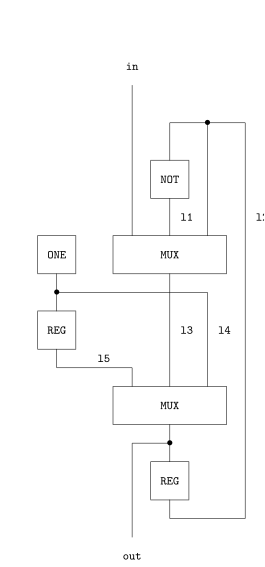
The devices making up this schematic will be modelled with
predicates (Gordon 1986). For example, the predicate
ONE is true of a signal out if for all times t the value of
out is T.
> Definition ONE_def: ONE(out:num->bool) = !t. out t = T
  End
Definition has been stored under "ONE_def"
val ONE_def = ⊢ ∀out. ONE out ⇔ ∀t. out t ⇔ T: thm
Note that, as discussed above, 'ONE_def' is used both as an ML
variable and as the name of the definition in the theory. Note
also how ':num->bool' has been added to resolve type
ambiguities; without this (or some other type information) the
typechecker would not be able to infer that t is to have type
num.
The binary predicate NOT is true of a pair of signals
(inp,out) if the value of out is always the negation of the
value of inp. Inverters are thus modelled as having no delay.
This is appropriate for a register-transfer level model, but not
at a lower level.
> Definition NOT_def:
     NOT(inp, out:num->bool) = !t. out t = ~(inp t)
  End
Definition has been stored under "NOT_def"
val NOT_def = ⊢ ∀inp out. NOT (inp,out) ⇔ ∀t. out t ⇔ ¬inp t: thm
The final combinational device needed is a multiplexer. This is
a ‘hardware conditional’; the input sw selects which of the
other two inputs are to be connected to the output out.
> Definition MUX_def:
    MUX(sw,in1,in2,out:num->bool) =
      !t. out t = if sw t then in1 t else in2 t
  End
Definition has been stored under "MUX_def"
val MUX_def =
   ⊢ ∀sw in1 in2 out.
       MUX (sw,in1,in2,out) ⇔ ∀t. out t ⇔ if sw t then in1 t else in2 t: thm
The remaining devices in the schematic are registers. These are
unit-delay elements; the values output at time t+1 are the
values input at the preceding time t, except at time 0 when
the register outputs F.3
> Definition REG_def:
    REG(inp,out:num->bool) =
       !t. out t = if (t=0) then F else inp(t-1)
  End
Definition has been stored under "REG_def"
val REG_def =
   ⊢ ∀inp out. REG (inp,out) ⇔ ∀t. out t ⇔ if t = 0 then F else inp (t − 1):
   thm
The schematic diagram above can be represented as a predicate by conjoining the relations holding between the various signals and then existentially quantifying the internal lines. This technique is explained elsewhere (e.g. see (Camilleri, Melham, and Gordon 1987; Gordon 1986)).
> Definition PARITY_IMP_def:
    PARITY_IMP(inp,out) =
      ?l1 l2 l3 l4 l5.
        NOT(l2,l1) /\ MUX(inp,l1,l2,l3) /\ REG(out,l2) /\
        ONE l4     /\ REG(l4,l5)        /\ MUX(l5,l3,l4,out)
  End
Definition has been stored under "PARITY_IMP_def"
val PARITY_IMP_def =
   ⊢ ∀inp out.
       PARITY_IMP (inp,out) ⇔
       ∃l1 l2 l3 l4 l5.
         NOT (l2,l1) ∧ MUX (inp,l1,l2,l3) ∧ REG (out,l2) ∧ ONE l4 ∧
         REG (l4,l5) ∧ MUX (l5,l3,l4,out): thm
Verification
The following theorem will eventually be proved:
|- !inp out. PARITY_IMP(inp,out) ==> (!t. out t = PARITY t inp)
This states that if inp and out are related as in the
schematic diagram (i.e. as in the definition of PARITY_IMP),
then the pair of signals (inp,out) satisfies the
specification.
First, the following lemma is proved; the correctness of the
parity checker follows from this and UNIQUENESS_LEMMA by the
transitivity of ==>.
> g ‘!inp out.
       PARITY_IMP(inp,out) ==>
       (out 0 = T) /\
       !t. out(SUC t) = if inp(SUC t) then ~(out t) else out t’;
val it =
   Proof manager status: 2 proofs.
   2. Completed goalstack:
        ⊢ ∀inp out.
            (out 0 ⇔ T) ∧
            (∀t. out (SUC t) ⇔ if inp (SUC t) then ¬out t else out t) ⇒
            ∀t. out t ⇔ PARITY t inp

   1. Incomplete goalstack:
        Initial goal:
        ∀inp out.
          PARITY_IMP (inp,out) ⇒
          (out 0 ⇔ T) ∧
          ∀t. out (SUC t) ⇔ if inp (SUC t) then ¬out t else out t
The first step in proving this goal is to rewrite with
definitions followed by a decomposition of the resulting goal
using strip_tac. The rewriting tactic PURE_REWRITE_TAC is
used; this does no built-in simplifications, only the ones
explicitly given in the list of theorems supplied as an argument.
One of the built-in simplifications used by REWRITE_TAC is
|- ~(x = T) = x. PURE_REWRITE_TAC is used to prevent
rewriting with this being done.
> e(PURE_REWRITE_TAC [PARITY_IMP_def, ONE_def, NOT_def,
                      MUX_def, REG_def] >>
    rpt strip_tac);
OK..
2 subgoals:
val it =

    0.  ∀t. l1 t ⇔ ¬l2 t
    1.  ∀t. l3 t ⇔ if inp t then l1 t else l2 t
    2.  ∀t. l2 t ⇔ if t = 0 then F else out (t − 1)
    3.  ∀t. l4 t ⇔ T
    4.  ∀t. l5 t ⇔ if t = 0 then F else l4 (t − 1)
    5.  ∀t. out t ⇔ if l5 t then l3 t else l4 t
   ------------------------------------
        out (SUC t) ⇔ if inp (SUC t) then ¬out t else out t

    0.  ∀t. l1 t ⇔ ¬l2 t
    1.  ∀t. l3 t ⇔ if inp t then l1 t else l2 t
    2.  ∀t. l2 t ⇔ if t = 0 then F else out (t − 1)
    3.  ∀t. l4 t ⇔ T
    4.  ∀t. l5 t ⇔ if t = 0 then F else l4 (t − 1)
    5.  ∀t. out t ⇔ if l5 t then l3 t else l4 t
   ------------------------------------
        out 0 ⇔ T
The top goal is the one printed last; its conclusion is
out 0 = T and its assumptions are equations relating the values
on the lines in the circuit. The natural next step would be to
expand the top goal by rewriting with the assumptions. However,
if this were done the system would go into an infinite loop
because the equations for out, l2 and l3 are mutually
recursive. Instead we use the first-order reasoner metis_tac
to do the work:
> e(metis_tac []);
OK..
metis: r[+0+17]+0+0+0+0+0+1+0+1#

Goal proved.
 [......] ⊢ out 0 ⇔ T

Remaining subgoals:
val it =

    0.  ∀t. l1 t ⇔ ¬l2 t
    1.  ∀t. l3 t ⇔ if inp t then l1 t else l2 t
    2.  ∀t. l2 t ⇔ if t = 0 then F else out (t − 1)
    3.  ∀t. l4 t ⇔ T
    4.  ∀t. l5 t ⇔ if t = 0 then F else l4 (t − 1)
    5.  ∀t. out t ⇔ if l5 t then l3 t else l4 t
   ------------------------------------
        out (SUC t) ⇔ if inp (SUC t) then ¬out t else out t
The first of the two subgoals is proved. Inspecting the
remaining goal it can be seen that it will be solved if its left
hand side, out(SUC t), is expanded using the assumption:
!t. out t = if l5 t then l3 t else l4 t
However, if this assumption is used for rewriting, then all the
subterms of the form out t will also be expanded. To prevent
this, we really want to rewrite with a formula that is
specifically about out (SUC t). We want to somehow pull the
assumption that we do have out of the list and rewrite with a
specialised version of it. We can do just this using
qpat_x_assum. This tactic is of type
term quotation -> thm -> tactic. It selects an assumption that
is of the form given by its first argument, and passes it to the
second argument, a function which expects a theorem and returns
a tactic. Here it is in action:
> e (qpat_x_assum ‘!t. out t = X t’
      (fn th => REWRITE_TAC [SPEC “SUC t” th]));
OK..
1 subgoal:
val it =

    0.  ∀t. l1 t ⇔ ¬l2 t
    1.  ∀t. l3 t ⇔ if inp t then l1 t else l2 t
    2.  ∀t. l2 t ⇔ if t = 0 then F else out (t − 1)
    3.  ∀t. l4 t ⇔ T
    4.  ∀t. l5 t ⇔ if t = 0 then F else l4 (t − 1)
   ------------------------------------
        (if l5 (SUC t) then l3 (SUC t) else l4 (SUC t)) ⇔
        if inp (SUC t) then ¬out t else out t
The pattern used here exploited something called higher order
matching. The actual assumption that was taken off the
assumption stack did not have a RHS that looked like the
application of a function (X in the pattern) to the t
parameter, but the RHS could nonetheless be seen as equal to the
application of some function to the t parameter. In fact,
the value that matched X was ``\x. if l5 x then l3 x else l4 x``.
Inspecting the goal above, it can be seen that the next step is
to unwind the equations for the remaining lines of the circuit.
We do using the standard simplifier rw.
> e (rw[]);
OK..   ... output elided ...

Goal proved.
 [......] ⊢ out (SUC t) ⇔ if inp (SUC t) then ¬out t else out t
val it =
   Initial goal proved.
   ⊢ ∀inp out.
       PARITY_IMP (inp,out) ⇒
       (out 0 ⇔ T) ∧ ∀t. out (SUC t) ⇔ if inp (SUC t) then ¬out t else out t
The theorem just proved is named PARITY_LEMMA and saved in the
current theory.
> val PARITY_LEMMA = top_thm ();
val PARITY_LEMMA =
   ⊢ ∀inp out.
       PARITY_IMP (inp,out) ⇒
       (out 0 ⇔ T) ∧ ∀t. out (SUC t) ⇔ if inp (SUC t) then ¬out t else out t:
   thm
PARITY_LEMMA could have been proved in one step with a single
compound tactic. Our initial goal can be expanded with a single
tactic corresponding to the sequence of tactics that were used
interactively:
> restart();   ... output elided ...
> e (PURE_REWRITE_TAC [PARITY_IMP_def, ONE_def, NOT_def,
                       MUX_def, REG_def] >>
    rpt strip_tac
    >- metis_tac []
    >- (qpat_x_assum ‘!t. out t = X t’
                 (fn th => REWRITE_TAC [SPEC “SUC t” th]) >>
        rw[]));
OK..
metis: r[+0+17]+0+0+0+0+0+1+0+1#
val it =
   Initial goal proved.
   ⊢ ∀inp out.
       PARITY_IMP (inp,out) ⇒
       (out 0 ⇔ T) ∧ ∀t. out (SUC t) ⇔ if inp (SUC t) then ¬out t else out t
Armed with PARITY_LEMMA, the final theorem is easily proved:
> Theorem PARITY_CORRECT:
    ∀inp out. PARITY_IMP(inp,out) ⇒ ∀t. out t = PARITY t inp
  Proof
    rpt strip_tac >> match_mp_tac UNIQUENESS_LEMMA >>
    irule PARITY_LEMMA >> rw[]
  QED
val PARITY_CORRECT =
   ⊢ ∀inp out. PARITY_IMP (inp,out) ⇒ ∀t. out t ⇔ PARITY t inp: thm
This completes the proof of the parity checking device.
Exercises
Two exercises are given in this section: Exercise 1 is straightforward, but Exercise 2 is quite tricky and might take a beginner several days to solve.
Exercise 1
Using only the devices ONE, NOT, MUX and REG defined in
Section 5.3, design and verify a register
RESET_REG with an input inp, reset line reset, output out
and behaviour specified as follows.
- If
resetisTat timet, then the value atoutat timetis alsoT. - If
resetisTat timetort+1, then the value output atoutat timet+1isT, otherwise it is equal to the value input at timetoninp.
This is formalized in HOL by the definition:
   RESET_REG(reset,inp,out) <=>
     (!t. reset t ==> (out t = T)) /\
     (!t. out(t+1) = if reset t \/ reset(t+1) then T else inp t)
Note that this specification is only partial; it doesn't specify
the output at time 0 in the case that there is no reset.
The solution to the exercise should be a definition of a
predicate RESET_REG_IMP as an existential quantification of a
conjunction of applications of ONE, NOT, MUX and REG to
suitable line names,4 together with a
proof of:
RESET_REG_IMP(reset,inp,out) ==> RESET_REG(reset,inp,out)
Exercise 2
-
Formally specify a resetable parity checker that has two boolean inputs
resetandinp, and one boolean outputoutwith the following behaviour:The value at
outisTif and only if there have been an even number ofTs input atinpsince the last time thatTwas input atreset. -
Design an implementation of this specification built using only the devices
ONE,NOT,MUXandREGdefined in Section 5.3. -
Verify the correctness of your implementation in HOL.
-
Signals are modelled as functions from numbers, representing times, to booleans. ↩
-
We'd like to use
inas one of our variable names, but this is a reserved word forlet-expressions. ↩ -
Time
0represents when the device is switched on. ↩ -
i.e. a definition of the same form as that of
PARITY_IMPon page \pageref{parity-imp}. ↩
Example: Combinatory Logic
Introduction
This small case study is a formalisation of (variable-free)
combinatory logic. This logic is of foundational importance in
theoretical computer science, and has a very rich theory. The
example builds principally on a development done by Tom Melham.
The complete script for the development is available as
clScript.sml in the examples/ind_def directory of the
distribution. It is self-contained and so includes the answers
to the exercises set at the end of this document.
The HOL sessions assume that the Unicode trace is on (as it is by default), meaning that even though the inputs may be written in pure ASCII, the output still uses nice Unicode output (symbols such as $\forall$ and $\Rightarrow$). The Unicode symbols could also be used in the input.
The type of combinators
The first thing we need to do is define the type of
combinators. There are just two of these, $\KC{}$ and $\SC$,
but we also need to be able to combine them, and for this we
need to introduce the notion of application. For lack of a
better ASCII symbol, we will use the hash (#) to represent this
in the logic. Finally, we will start by “hiding” the names S
and K so that the constants of these names from the existing
HOL theories won't interfere with parsing.
> hide "K"; hide "S";   ... output elided ...
> Datatype: cl = K | S | # cl cl
  End
<<HOL message: Defined type: "cl">>
We also want the # to be an infix, so we set its fixity to be a
tight left-associative infix:
> set_fixity "#" (Infixl 1100);
val it = (): unit
Combinator reductions
Combinatory logic is the study of how values of this type can evolve given various rules describing how they change. Therefore, our next step is to define the reductions that combinators can undergo. There are two basic rules:
$$\begin{array}{lcl} \KC\;x\;y & \rightarrow & x\\ \SC\;f\;g\;x & \rightarrow & (f\,x)(g\,x) \end{array}$$
Here, in our description outside of HOL, we use juxtaposition
instead of the #. Further, juxtaposition is also
left-associative, so that $\con{K}\;x\;y$ should be read as
$\con{K}\;\#\;x\;\#\;y$ which is in turn
$(\con{K}\;\#\;x)\;\#\;y$.
Given a term in the logic, we want these reductions to be able to fire at any point, not just at the top level, so we need two further congruence rules:
$$ \begin{array}{c} \dfrac{x\;\;\rightarrow\;\;x'}{x\;y\;\;\rightarrow\;\;x'\;y} \qquad \dfrac{y\;\;\rightarrow\;\;y'}{x\;y\;\;\rightarrow\;\;x\;y'} \end{array} $$
In HOL, we can capture this relation with an inductive
definition. First we need to set our arrow symbol up as an infix
to make everything that bit prettier. The set_mapped_fixity
function lets the arrow be our surface syntax, but maps to the
name redn underneath. Making constants have pure alphanumeric
names is generally a good idea.
> set_mapped_fixity {fixity = Infix(NONASSOC, 450),
                     tok = "-->", term_name = "redn"};
val it = (): unit
We make our arrow symbol non-associative, thereby making it a
parse error to write x --> y --> z. It would be nice to be
able to write this and have it mean x --> y /\ y --> z, but
this is not presently possible with the HOL parser.
Our next step is to actually define the relation, using the
Inductive syntax. Using the provided stem redn as a base,
the underlying facility proves a number of theorems for us, and
shows us three: redn_rules, redn_ind, redn_cases. These
theorems are available in the ML session under those names, and
are also saved under those names when the theory is exported.
> Inductive redn:
    (!x y f. x --> y   ==>    f # x --> f # y) /\
    (!f g x. f --> g   ==>    f # x --> g # x) /\
    (!x y.   K # x # y --> x) /\
    (!f g x. S # f # g # x --> (f # x) # (g # x))
  End
val redn_cases =
   ⊢ ∀a0 a1.
       a0 --> a1 ⇔
       (∃x y f. a0 = f # x ∧ a1 = f # y ∧ x --> y) ∨
       (∃f g x. a0 = f # x ∧ a1 = g # x ∧ f --> g) ∨ (∃y. a0 = K # a1 # y) ∨
       ∃f g x. a0 = S # f # g # x ∧ a1 = f # x # (g # x): thm
val redn_ind =
   ⊢ ∀redn'.
       (∀x y f. redn' x y ⇒ redn' (f # x) (f # y)) ∧
       (∀f g x. redn' f g ⇒ redn' (f # x) (g # x)) ∧
       (∀x y. redn' (K # x # y) x) ∧
       (∀f g x. redn' (S # f # g # x) (f # x # (g # x))) ⇒
       ∀a0 a1. a0 --> a1 ⇒ redn' a0 a1: thm
val redn_rules =
   ⊢ (∀x y f. x --> y ⇒ f # x --> f # y) ∧
     (∀f g x. f --> g ⇒ f # x --> g # x) ∧ (∀x y. K # x # y --> x) ∧
     ∀f g x. S # f # g # x --> f # x # (g # x): thm
Using the redn_rules theorem we can demonstrate single steps of
our reduction relation:
> PROVE [redn_rules] ``S # (K # x # x) --> S # x``;
Meson search level:
...val it = ⊢ S # (K # x # x) --> S # x: thm
The system we have just defined is as powerful as the $\lambda$-calculus, Turing machines, and all the other standard models of computation.
One useful result about the combinatory logic is that it is confluent. Consider the term $\SC\;z\;(\KC\;\KC)\;(\KC\;y\;x)$. It can make two reductions, to $\SC\;z\;(\KC\;\KC)\;y$ and also to $(z\;(\KC\;y\;x))\,(\KC\;\KC\;(\KC\;y\;x))$. Do these two choices of reduction mean that from this point on the terms have two completely separate histories? Roughly speaking, to be confluent means that the answer to this question is no.
Transitive closure and confluence
A notion crucial to that of confluence is that of transitive closure. We have defined a system that evolves by specifying how an algebraic value can evolve into possible successor values in one step. The natural next question is to ask for a characterisation of evolution over one or more steps of the $\rightarrow$ relation.
In fact, we will define a relation that holds between two values if the second can be reached from the first in zero or more steps. This is the reflexive, transitive closure of our original relation. However, rather than tie our new definition to our original relation, we will develop this notion independently and prove a variety of results that are true of any system, not just our system of combinatory logic.
So, we begin our abstract digression with another inductive
definition. Our new constant is $\con{RTC}$, such that
$\con{RTC}\;R\;x\;y$ is true if it is possible to get from $x$
to $y$ with zero or more “steps” of the $R$ relation. (The
standard notation for $\con{RTC}\;R$ is $R^*$; we will see HOL
try to approximate this with the text R^*.) We can express
this idea with just two rules. The first
$$\dfrac{}{\con{RTC}\;R\;x\;x}$$
says that it's always possible to get from $x$ to $x$ in zero or more steps. The second
$$\dfrac{R\;x\;y \qquad \con{RTC}\;R\;y\;z}{\con{RTC}\;R\;x\;z}$$
says that if you can take a single step from $x$ to $y$, and then take zero or more steps to get $y$ to $z$, then it's possible to take zero or more steps to get between $x$ and $z$. The realisation of these rules in HOL is again straightforward.
(As it happens, $\con{RTC}$ is already a defined constant in the
context we're working in (it is found in relationTheory), so
we'll hide it from view before we begin. We thus avoid messages
telling us that we are inputting ambiguous terms. The
ambiguities would always be resolved in the favour of more
recent definition, but the warnings are annoying. We inherit
the nice syntax for the old constant with our new one.)
> val _ = hide "RTC";

> Inductive RTC:
   (!x.     RTC R x x) /\
   (!x y z. R x y /\ RTC R y z ==> RTC R x z)
  End
<<HOL message: inventing new type variable names: 'a>>
<<HOL message: Treating "R" as schematic variable>>
val RTC_cases = ⊢ ∀R a0 a1. R꙳ a0 a1 ⇔ a1 = a0 ∨ ∃y. R a0 y ∧ R꙳ y a1: thm
val RTC_ind =
   ⊢ ∀R RTC'.
       (∀x. RTC' x x) ∧ (∀x y z. R x y ∧ RTC' y z ⇒ RTC' x z) ⇒
       ∀a0 a1. R꙳ a0 a1 ⇒ RTC' a0 a1: thm
val RTC_rules = ⊢ ∀R. (∀x. R꙳ x x) ∧ ∀x y z. R x y ∧ R꙳ y z ⇒ R꙳ x z: thm
Now let us go back to the notion of confluence. We want this to mean something like: “though a system may take different paths in the short-term, those two paths can always end up in the same place”. This suggests that we define confluent thus:
> Definition confluent_def:
    confluent R =
      !x y z. RTC R x y /\ RTC R x z ==>
              ?u. RTC R y u /\ RTC R z u
  End
<<HOL message: inventing new type variable names: 'a>>
Definition has been stored under "confluent_def"
val confluent_def =
   ⊢ ∀R. confluent R ⇔ ∀x y z. R꙳ x y ∧ R꙳ x z ⇒ ∃u. R꙳ y u ∧ R꙳ z u: thm
This property states of $R$ that we can “complete the diamond”; if we have

then we can complete with a fresh value $u$:

One nice property of confluent relations is that from any one starting point they produce no more than one normal form, where a normal form is a value from which no further steps can be taken.
> Definition normform_def:  normform R x = !y. ~R x y
  End
<<HOL message: inventing new type variable names: 'a, 'b>>
Definition has been stored under "normform_def"
val normform_def = ⊢ ∀R x. normform R x ⇔ ∀y. ¬R x y: thm
In other words, a system has an $R$-normal form at $x$ if there
are no connections via $R$ to any other values. (We could have
written ~?y. R x y as our RHS for the definition above.)
We can now prove the following:
> g `!R. confluent R ==>
         !x y z.
           RTC R x y /\ normform R y /\
           RTC R x z /\ normform R z ==> (y = z)`;
<<HOL message: inventing new type variable names: 'a>>
val it =
   Proof manager status: 1 proof.
   1. Incomplete goalstack:
        Initial goal:
        ∀R. confluent R ⇒
            ∀x y z. R꙳ x y ∧ normform R y ∧ R꙳ x z ∧ normform R z ⇒ y = z
We rewrite with the definition of confluence:
> e (rw[confluent_def]);
OK..
1 subgoal:
val it =

    0.  ∀x y z. R꙳ x y ∧ R꙳ x z ⇒ ∃u. R꙳ y u ∧ R꙳ z u
    1.  R꙳ x y
    2.  normform R y
    3.  R꙳ x z
    4.  normform R z
   ------------------------------------
        y = z
Our confluence property is now assumption 0, and we can use it to infer that there is a $u$ at the base of the diamond:
> e (`?u. RTC R y u /\ RTC R z u` by metis_tac []);
OK..
metis: r[+0+8]+0+0+0+0+0+0+1+1+1+1#
1 subgoal:
val it =

    0.  ∀x y z. R꙳ x y ∧ R꙳ x z ⇒ ∃u. R꙳ y u ∧ R꙳ z u
    1.  R꙳ x y
    2.  normform R y
    3.  R꙳ x z
    4.  normform R z
    5.  R꙳ y u
    6.  R꙳ z u
   ------------------------------------
        y = z
So, from $y$ we can take zero or more steps to get to $u$ and similarly from $z$. But, we also know that we're at an $R$-normal form at both $y$ and $z$. We can't take any steps at all from these values. We can conclude both that $u = y$ and $u = z$, and this in turn means that $y = z$, which is our goal. So we can finish with
> e (metis_tac [normform_def, RTC_cases]);
OK..
metis: r[+0+20]+0+0+0+0+0+0+0+0+0+0+0+0+6+0+0+0+0+0+0+2+0 .... #   ... output elided ...

Goal proved.
 [.....] ⊢ y = z
val it =
   Initial goal proved.
   ⊢ ∀R. confluent R ⇒
         ∀x y z. R꙳ x y ∧ normform R y ∧ R꙳ x z ∧ normform R z ⇒ y = z: proof
Packaged up so as to remove the sub-goal package commands, we can prove and save the theorem for future use by:
> Theorem confluent_normforms_unique:
    !R. confluent R ==>
        !x y z. RTC R x y /\ normform R y /\
                RTC R x z /\ normform R z ==> y = z
  Proof
    rw[confluent_def] >>
    `?u. RTC R y u /\ RTC R z u` by metis_tac [] >>
    metis_tac [normform_def, RTC_cases]
  QED
<<HOL message: inventing new type variable names: 'a>>
metis: r[+0+8]+0+0+0+0+0+0+1+1+1+1#
metis: r[+0+20]+0+0+0+0+0+0+0+0+0+0+0+0+6+0+0+0+0+0+0+2+0 .... #
val confluent_normforms_unique =
   ⊢ ∀R. confluent R ⇒
         ∀x y z. R꙳ x y ∧ normform R y ∧ R꙳ x z ∧ normform R z ⇒ y = z: thm
⋯⋄⋯
Clearly confluence is a nice property for a system to have. The question is how we might manage to prove it. Let's start by defining the diamond property that we used in the definition of confluence. We'll again hide the existing definition of “diamond”:
> val _ = hide "diamond";
> Definition diamond_def:
    diamond R = !x y z. R x y /\ R x z ==> ?u. R y u /\ R z u
  End
<<HOL message: inventing new type variable names: 'a>>
Definition has been stored under "diamond_def"
val diamond_def =
   ⊢ ∀R. diamond R ⇔ ∀x y z. R x y ∧ R x z ⇒ ∃u. R y u ∧ R z u: thm
Now we clearly have that confluence of a relation is equivalent to the reflexive, transitive closure of that relation having the diamond property.
> Theorem confluent_diamond_RTC:
     !R. confluent R = diamond (RTC R)
  Proof   rw[confluent_def, diamond_def]
  QED
<<HOL message: inventing new type variable names: 'a>>
val confluent_diamond_RTC = ⊢ ∀R. confluent R ⇔ diamond R꙳: thm
So far so good. How then do we show the diamond property for $\con{RTC}\;R$? The answer that leaps to mind is to hope that if the original relation has the diamond property, then maybe the reflexive and transitive closure will too. The theorem we want is
$$\con{diamond}\;R \;\Rightarrow\; \con{diamond}\,(\con{RTC}\;R)$$
Graphically, this is hoping that from $x$ with single $R$-arrows
to $y$ (left) and $z$ (right), and a destination $u$ reachable
from both $y$ and $z$ (the small diamond), we will be able to
conclude that with two RTC R-paths from $x$ to $p$ and from
$x$ to $q$, the diamond can be completed: there is some $r$
reachable from both $p$ and $q$ via $\con{RTC}\;R$ paths going
through $u$. The presence of two instances of $\con{RTC}\;R$ is
an indication that this proof will require two inductions. With
the first we will prove the “lop-sided” version: if $x$ takes
one step in one direction (to $z$) and many steps in another (to
$p$), then the diamond property for $R$ will guarantee us the
existence of $r$, to which we will be able to take many steps
from both $p$ and $z$.
We state the goal so we can easily strip away the outermost assumption (that $R$ has the diamond property) before beginning the rule induction.1
> g `!R. diamond R ==>
         !x p z. RTC R x p /\ R x z ==>
                 ?u. RTC R p u /\ RTC R z u`;
<<HOL message: inventing new type variable names: 'a>>
val it =
   Proof manager status: 1 proof.
   1. Incomplete goalstack:
        Initial goal:
        ∀R. diamond R ⇒ ∀x p z. R꙳ x p ∧ R x z ⇒ ∃u. R꙳ p u ∧ R꙳ z u
First, we strip away the diamond property assumption (two things
need to be stripped: the outermost universal quantifier and the
antecedent of the implication). If we use rw at this point,
we strip away too much so we have to be more precise and use the
lower level tool strip_tac. This tactic will remove a
universal quantification, an implication or a conjunction:
> e (strip_tac >> strip_tac);
OK..
1 subgoal:
val it =

    0.  diamond R
   ------------------------------------
        ∀x p z. R꙳ x p ∧ R x z ⇒ ∃u. R꙳ p u ∧ R꙳ z u
Now we can use the induction principle for reflexive and
transitive closure (alternatively, we perform a “rule
induction”). To do this, we use the Induct_on command that is
also used to do structural induction on algebraic data types
(such as numbers and lists). We provide the name of the
constant whose induction principle we want to use, and the
tactic does the rest:
> e (Induct_on `RTC`);
OK..
1 subgoal:
val it =

    0.  diamond R
   ------------------------------------
        (∀x z. R x z ⇒ ∃u. R꙳ x u ∧ R꙳ z u) ∧
        ∀x x' p.
          R x x' ∧ R꙳ x' p ∧ (∀z. R x' z ⇒ ∃u. R꙳ p u ∧ R꙳ z u) ⇒
          ∀z. R x z ⇒ ∃u. R꙳ p u ∧ R꙳ z u
Let's strip the goal as much as possible with the aim of making what remains to be proved easier to see:
> e (rw[]);
OK..
2 subgoals:
val it =

    0.  diamond R
    1.  R x x'
    2.  R꙳ x' p
    3.  ∀z. R x' z ⇒ ∃u. R꙳ p u ∧ R꙳ z u
    4.  R x z
   ------------------------------------
        ∃u. R꙳ p u ∧ R꙳ z u

    0.  diamond R
    1.  R x z
   ------------------------------------
        ∃u. R꙳ x u ∧ R꙳ z u
This first goal is easy. It corresponds to the case where the
many steps from $x$ to $p$ are actually no steps at all, and $p$
and $x$ are actually the same place. In the other direction,
$x$ has taken one step to $z$, and we need to find somewhere
reachable in zero or more steps from both $x$ and $z$. Given
what we know so far, the only candidate is $z$ itself. In fact,
we don't even need to provide this witness explicitly:
metis_tac will find it for us, as long as we tell it what the
rules governing $\con{RTC}$ are:
> e (metis_tac [RTC_rules]);
OK..
metis: r[+0+9]+0+0+0+0+0+0+1+0+0+6+1#

Goal proved.
 [..] ⊢ ∃u. R꙳ x u ∧ R꙳ z u

Remaining subgoals:
val it =

    0.  diamond R
    1.  R x x'
    2.  R꙳ x' p
    3.  ∀z. R x' z ⇒ ∃u. R꙳ p u ∧ R꙳ z u
    4.  R x z
   ------------------------------------
        ∃u. R꙳ p u ∧ R꙳ z u
And what of this remaining goal? Assumptions one and four between them are the top of an $R$-diamond. Let's use the fact that we have the diamond property for $R$ and infer that there exists a $v$ to which $x'$ and $z$ can both take single steps:
> e (`?v. R x' v /\ R z v` by metis_tac [diamond_def]);
OK..
metis: r[+0+16]+0+0+0+0+0+0+0+0+0+0+0+0+0+1+1+1+1+1#
1 subgoal:
val it =

    0.  diamond R
    1.  R x x'
    2.  R꙳ x' p
    3.  ∀z. R x' z ⇒ ∃u. R꙳ p u ∧ R꙳ z u
    4.  R x z
    5.  R x' v
    6.  R z v
   ------------------------------------
        ∃u. R꙳ p u ∧ R꙳ z u
Now we can apply our induction hypothesis (assumption 3) to
complete the long, lop-sided strip of the diamond. We will
conclude that there is a $u$ such that $R^*\;p\;u$ and
$R^*\;v\;u$. We actually need a $u$ such that
$\con{RTC}\;R\;z\;u$, but because there is a single $R$-step
between $z$ and $v$ we have that as well. All we need to provide
metis_tac is the rules for $\con{RTC}$:
> e (metis_tac [RTC_rules]);
OK..
metis: r[+0+15]+0+0+0+0+0+0+0+0+0+0+1+0+0+1+0+1+0+10+2+0+ .... #   ... output elided ...

Goal proved.
 [.] ⊢ ∀x p z. R꙳ x p ∧ R x z ⇒ ∃u. R꙳ p u ∧ R꙳ z u
val it =
   Initial goal proved.
   ⊢ ∀R. diamond R ⇒ ∀x p z. R꙳ x p ∧ R x z ⇒ ∃u. R꙳ p u ∧ R꙳ z u: proof
Again we can (and should) package up the lemma, avoiding the sub-goal package commands:
Theorem R_RTC_diamond:
  !R. diamond R ⇒
      !x p z. RTC R x p ∧ R x z ⇒
              ∃u. RTC R p u ∧ RTC R z u
Proof
  strip_tac >> strip_tac >> Induct_on `RTC` >> rw[]
  >- metis_tac [RTC_rules]
  >- (`?v. R x' v /\ R z v` by metis_tac [diamond_def] >>
      metis_tac [RTC_rules])
QED
⋯⋄⋯
Now we can move on to proving that if $R$ has the diamond property, so too does $R^*$. We want to prove this by induction again. We state the goal as the obvious
$$\con{diamond}\;R\;\Rightarrow\;\con{diamond}\,(R^*)$$
expecting to strip away the LHS of the goal as an assumption
(which will feed into the lemma we just proved), and to perform
another “RTC-induction” on what the second diamond expands
into:
> g `!R. diamond R ==> diamond (RTC R)`;
<<HOL message: inventing new type variable names: 'a>>
val it =
   Proof manager status: 1 proof.
   1. Incomplete goalstack:
        Initial goal:
        ∀R. diamond R ⇒ diamond R꙳
So, we begin by stripping away the diamond property assumption.
Then, we expand with the definition of diamond in the goal.
> e (strip_tac >> strip_tac >> simp[diamond_def]);
OK..
1 subgoal:
val it =

    0.  diamond R
   ------------------------------------
        ∀x y z. R꙳ x y ∧ R꙳ x z ⇒ ∃u. R꙳ y u ∧ R꙳ z u
We see that the simplifier has kept the diamond-assumption
untouched, but has exposed two RTC terms in the goal. In
order to make it clear that we wish to induct on the first, we
can write a more elaborate pattern when we induct:
> e (Induct_on `RTC R x y` >> rw[]);
OK..
2 subgoals:
val it =

    0.  diamond R
    1.  R x x'
    2.  R꙳ x' y
    3.  ∀z. R꙳ x' z ⇒ ∃u. R꙳ y u ∧ R꙳ z u
    4.  R꙳ x z
   ------------------------------------
        ∃u. R꙳ y u ∧ R꙳ z u

    0.  diamond R
    1.  R꙳ x z
   ------------------------------------
        ∃u. R꙳ x u ∧ R꙳ z u
The first goal is again an easy one, corresponding to the case where the trip from $x$ to $y$ has been one of no steps whatsoever.
> e (metis_tac [RTC_rules]);
OK..
metis: r[+0+9]+0+0+0+0+0+0+1#

Goal proved.
 [..] ⊢ ∃u. R꙳ x u ∧ R꙳ z u

Remaining subgoals:
val it =

    0.  diamond R
    1.  R x x'
    2.  R꙳ x' y
    3.  ∀z. R꙳ x' z ⇒ ∃u. R꙳ y u ∧ R꙳ z u
    4.  R꙳ x z
   ------------------------------------
        ∃u. R꙳ y u ∧ R꙳ z u
This goal is very similar to the one we saw earlier. We have the top of a (“lop-sided”) diamond in assumptions 1 and 4, so we can infer the existence of a common destination for $x'$ and $z$:
> e (`?v. RTC R x' v /\ RTC R z v` by metis_tac [R_RTC_diamond]);
OK..
metis: r[+0+13]+0+0+0+0+0+0+0+1+0+0+0+1+0+1+1+1+0+1+1#
1 subgoal:
val it =

    0.  diamond R
    1.  R x x'
    2.  R꙳ x' y
    3.  ∀z. R꙳ x' z ⇒ ∃u. R꙳ y u ∧ R꙳ z u
    4.  R꙳ x z
    5.  R꙳ x' v
    6.  R꙳ z v
   ------------------------------------
        ∃u. R꙳ y u ∧ R꙳ z u
At this point in the last proof we were able to finish it all
off by just appealing to the rules for $\con{RTC}$. This time
it is not quite so straightforward. When we use the induction
hypothesis (assumption 3), we can conclude that there is a $u$
to which both $y$ and $v$ can connect in zero or more steps, but
in order to show that this $u$ is reachable from $z$, we need to
be able to conclude $R^*\;z\;u$ when we know that $R^*\;z\;v$
(assumption 6 above) and $R^*\;v\;u$ (our consequence of the
inductive hypothesis). We leave the proof of this general
result as an exercise, and here assume that it is already proved
as the theorem RTC_RTC.
> e (metis_tac [RTC_rules, RTC_RTC]);
OK..
metis: r[+0+16]+0+0+0+0+0+0+0+0+0+0+2+0+0+0+0+1+14+21+1+2 .... #   ... output elided ...

Goal proved.
 [.] ⊢ ∀x y z. R꙳ x y ∧ R꙳ x z ⇒ ∃u. R꙳ y u ∧ R꙳ z u
val it =
   Initial goal proved.
   ⊢ ∀R. diamond R ⇒ diamond R꙳: proof
We can now package up our desired result:
Theorem diamond_RTC:
  !R. diamond R ==> diamond (RTC R)
Proof
  strip_tac >> strip_tac >> simp[diamond_def] >>
  Induct_on `RTC R x y` >> rw[]
  >-  metis_tac[RTC_rules]
  >- (`?v. RTC R x' v /\ RTC R z v` by metis_tac[R_RTC_diamond] >>
      metis_tac [RTC_RTC, RTC_rules])
QED
Back to combinators
Now, we are in a position to return to the real object of study and prove confluence for combinatory logic. We have done an abstract development and established that
$$ \begin{array}{rcl} \con{diamond}\;R & \Rightarrow & \con{diamond}\,(\con{RTC}\;R)\\ \con{diamond}\,(\con{RTC}\;R) & \equiv & \con{confluent}\;R\\ \end{array} $$
(We have also established a couple of other useful results along the way.)
Sadly, it just isn't the case that $\rightarrow$, our one-step relation for combinators, has the diamond property. A counter-example is $\KC\;\SC\;(\KC\;\KC\;\KC)$. Its possible evolution can be described graphically: $\KC\;\SC\;(\KC\;\KC\;\KC)$ reduces both to $\SC$ (by the outer $\KC\;x\;y\to x$ rule, with $x = \SC$ and $y = \KC\;\KC\;\KC$) and to $\KC\;\SC\;\KC$ (by the inner $\KC$-redex $\KC\;\KC\;\KC\to\KC$). The latter then reduces to $\SC$ as well.
If we had the diamond property, it should be possible to find a common destination for $\KC\;\SC\;\KC$ and $\SC$. However, $\SC$ doesn't admit any reductions whatsoever, so there isn't a common destination.2
This is a problem. We are going to have to take another approach. We will define another reduction strategy (parallel reduction), and prove that its reflexive, transitive closure is actually the same relation as our original's reflexive and transitive closure. Then we will also show that parallel reduction has the diamond property. This will establish that its reflexive, transitive closure has it too. Then, because they are the same relation, we will have that the reflexive, transitive closure of our original relation has the diamond property, and therefore, our original relation will be confluent.
Parallel reduction
Our new relation allows for any number of reductions to occur in
parallel. We use the -||-> symbol to indicate parallel
reduction because of its own parallel lines, and use predn to
name the constant:
> set_mapped_fixity {tok = "-||->", fixity = Infix(NONASSOC, 450),
                     term_name = "predn"};
val it = (): unit
Then we can define parallel reduction itself. The rules look very similar to those for $\rightarrow$. The difference is that we allow the reflexive transition, and say that an application of $x\;u$ can be transformed to $y\;v$ if there are transformations taking $x$ to $y$ and $u$ to $v$. This is why we must have reflexivity incidentally. Without it, a term like $(\KC\;x\;y)\,\KC$ couldn't reduce because while the LHS of the application ($\KC\;x\;y$) can reduce, its RHS ($\KC$) can't.
> Inductive predn:
    (!x. x -||-> x) /\
    (!x y u v. x -||-> y /\ u -||-> v
                      ==>
               x # u -||-> y # v) /\
    (!x y. K # x # y -||-> x) /\
    (!f g x. S # f # g # x -||-> (f # x) # (g # x))
  End   ... output elided ...
Using RTC
Now we can set up nice syntax for the reflexive and transitive
closures of our two relations. We will use ASCII symbols for
both that consist of the original symbol followed by an
asterisk. Note also how, in defining the two relations, we have
to use the $ character to “escape” the symbols' usual
fixities. This is exactly analogous to the way in which ML's
op keyword is used. First, we create the desired symbol for
the concrete syntax, and then we “overload” it so that the
parser will expand it to the desired form.
> set_fixity "-->*" (Infix(NONASSOC, 450));
val it = (): unit

> Overload "-->*" = “RTC redn”;
We do exactly the same thing for the reflexive and transitive closure of our parallel reduction.
> set_fixity "-||->*" (Infix(NONASSOC, 450));
val it = (): unit

> Overload "-||->*" = ``RTC predn``;
Incidentally, in conjunction with PROVE we can now
automatically demonstrate relatively long chains of reductions:
> PROVE [RTC_rules, redn_rules] ``S # K # K # x -->* x``;
Meson search level:
......val it = ⊢ S # K # K # x -->* x: thm

> PROVE [RTC_rules, redn_rules]
   ``S # (S # (K # S) # K) # (S # K # K) # f # x -->*
     f # (f # x)``;
Meson search level:
...........................val it = ⊢ S # (S # (K # S) # K) # (S # K # K) # f # x -->* f # (f # x): thm
(The latter sequence is seven reductions long.)
Proving the RTCs are the same
We start with the easier direction, and show that everything in $\rightarrow^*$ is in $\mathpredn^*$. Because $\con{RTC}$ is monotone (which fact is left to the reader to prove), we can reduce this to showing that $x\rightarrow y\Rightarrow x\mathpredn y$.
Our goal:
> g `!x y. x -->* y ==> x -||->* y`;
val it =
   Proof manager status: 1 proof.
   1. Incomplete goalstack:
        Initial goal:
        ∀x y. x -->* y ⇒ x -||->* y
We back-chain using our monotonicity result:
> e (match_mp_tac RTC_monotone);
OK..
1 subgoal:
val it =

   ∀x y. x --> y ⇒ x -||-> y
Now we can induct over the rules for $\rightarrow$:
> e (Induct_on `x --> y`);
OK..
1 subgoal:
val it =

   (∀x y f. x --> y ∧ x -||-> y ⇒ f # x -||-> f # y) ∧
   (∀f g x. f --> g ∧ f -||-> g ⇒ f # x -||-> g # x) ∧
   (∀x y. K # x # y -||-> x) ∧ ∀f g x. S # f # g # x -||-> f # x # (g # x)
We could split the 4-way conjunction apart into four goals, but there is no real need. It is quite clear that each follows immediately from the rules for parallel reduction.
> e (metis_tac [predn_rules]);
OK..
metis: r[+0+5]#
r[+0+4]#
r[+0+8]+0+0+0+0+0+0+0+1#
r[+0+8]+0+0+0+0+0+0+0+1#   ... output elided ...

Goal proved.
⊢ ∀x y. x --> y ⇒ x -||-> y
val it =
   Initial goal proved.
   ⊢ ∀x y. x -->* y ⇒ x -||->* y: proof
Packaged into a tidy little sub-goal-package-free parcel, our proof is
Theorem RTCredn_RTCpredn:
  !x y. x -->* y   ==>   x -||->* y
Proof
  match_mp_tac RTC_monotone >>
  Induct_on `x --> y` >> metis_tac [predn_rules]
QED
⋯⋄⋯
Our next proof is in the other direction. It should be clear that we will not just be able to appeal to the monotonicity of $\con{RTC}$ this time; one step of the parallel reduction relation can not be mirrored with one step of the original reduction relation. It's clear that mirroring one step of the parallel reduction relation might take many steps of the original relation. Let's prove that then:
> g `!x y. x -||-> y   ==>   x -->* y`;
val it =
   Proof manager status: 1 proof.
   1. Incomplete goalstack:
        Initial goal:
        ∀x y. x -||-> y ⇒ x -->* y
This time our induction will be over the rules defining the parallel reduction relation.
> e (Induct_on `x -||-> y`);
OK..
1 subgoal:
val it =

   (∀x. x -->* x) ∧
   (∀x y x' y'.
      x -||-> y ∧ x -->* y ∧ x' -||-> y' ∧ x' -->* y' ⇒ x # x' -->* y # y') ∧
   (∀y y'. K # y # y' -->* y) ∧ ∀f g x. S # f # g # x -->* f # x # (g # x)
There are four conjuncts here, and it should be clear that all
but the second can be proved immediately by appeal to the rules
for the transitive closure and for $\rightarrow$ itself. So, we
split apart the conjunctions, use a THEN1 to discharge the
first subgoal, thus putting the second subgoal into focus to be
dealt with more carefully. Note that >- is sugar for THEN1.
> e (rpt conj_tac >- metis_tac[RTC_rules, redn_rules]);
OK..
metis: r[+0+3]#
3 subgoals:
val it =

   ∀f g x. S # f # g # x -->* f # x # (g # x)

   ∀y y'. K # y # y' -->* y

   ∀x y x' y'.
     x -||-> y ∧ x -->* y ∧ x' -||-> y' ∧ x' -->* y' ⇒ x # x' -->* y # y'
What of this sub-goal? If we look at it for long enough, we
should see that it is another monotonicity fact. More
accurately, we need what is called a congruence result for
-->*. In this form, it's not quite right for easy proof.
Let's go away and prove RTCredn_ap_monotonic separately.
(Another exercise!) Our new theorem should state
Theorem RTCredn_ap_congruence:
  !x y. x -->* y ==> !z. x # z -->* y # z /\ z # x -->* z # y
Proof  ...
QED
Now that we have this, our sub-goal is almost immediately provable. Using it, we know that
$$ \begin{array}{c} x\;x' \rightarrow^* y\;x' \\ y\;x' \rightarrow^* y\;y' \end{array} $$
All we need to do is “stitch together” the two transitions above
and go from $x\;x'$ to $y\;y'$. We can do this by appealing to
our earlier RTC_RTC result.
> e (metis_tac [RTC_RTC, RTCredn_ap_congruence]);
OK..
metis: r[+0+9]+0+0+0+0+0+0+0+0+10+1+3+1+3+1+7+1+1#

Goal proved.
⊢ ∀x y x' y'.
    x -||-> y ∧ x -->* y ∧ x' -||-> y' ∧ x' -->* y' ⇒ x # x' -->* y # y'

Remaining subgoals:
val it =

   ∀f g x. S # f # g # x -->* f # x # (g # x)

   ∀y y'. K # y # y' -->* y
But given that we can finish off what we thought was an awkward
branch with just another application of metis_tac, we don't
need to use our fancy branching footwork at the stage before.
Instead, we can just merge the theorem lists passed to both
invocations, dispense with the rpt conj_tac and have a very
short tactic proof indeed:
Theorem predn_RTCredn:
  !x y. x -||-> y  ==>  x -->* y
Proof
  Induct_on `x -||-> y` >>
  metis_tac [RTC_rules, redn_rules, RTC_RTC,
             RTCredn_ap_congruence]
QED
⋯⋄⋯
Now it's time to prove that if a number of parallel reduction steps are chained together, then we can mirror this with some number of steps using the original reduction relation. Our goal:
> g `!x y. x -||->* y  ==> x -->* y`;
val it =
   Proof manager status: 1 proof.
   1. Incomplete goalstack:
        Initial goal:
        ∀x y. x -||->* y ⇒ x -->* y
We use the appropriate induction principle to get to:
> e (Induct_on `RTC`);
OK..
1 subgoal:
val it =

   (∀x. x -->* x) ∧ ∀x x' y. x -||-> x' ∧ x' -||->* y ∧ x' -->* y ⇒ x -->* y
This we can finish off in one step. The first conjunct is
obvious, and in the second the x -||-> y and our last result
combine to tell us that x -->* y. Then this can be chained
together with the other assumption in the second conjunct and
we're done.
> e (metis_tac [RTC_rules, predn_RTCredn, RTC_RTC]);
OK..
metis: r[+0+12]+0+0+0+0+0+0+0+0+1+0+0+8+12+5+0+0+3+4+4+8+1#
r[+0+3]#

Goal proved.
⊢ (∀x. x -->* x) ∧ ∀x x' y. x -||-> x' ∧ x' -||->* y ∧ x' -->* y ⇒ x -->* y
val it =
   Initial goal proved.
   ⊢ ∀x y. x -||->* y ⇒ x -->* y: proof
Packaged up, this proof is:
Theorem RTCpredn_RTCredn:
  !x y. x -||->* y   ==>  x -->* y
Proof
  Induct_on `RTC` >>
  metis_tac [predn_RTCredn, RTC_RTC, RTC_rules]
QED
⋯⋄⋯
Our final act is to use what we have so far to conclude that $\rightarrow^*$ and $\mathpredn^*$ are equal. We state our goal:
> g `$-||->* = $-->*`;
val it =
   Proof manager status: 1 proof.
   1. Incomplete goalstack:
        Initial goal:
        $-||->* = $-->*
We want to now appeal to extensionality. The simplest way to do
this is to rewrite with the theorem FUN_EQ_THM:
> FUN_EQ_THM;
val it = ⊢ ∀f g. f = g ⇔ ∀x. f x = g x: thm
So, we rewrite:
> e (rw[FUN_EQ_THM]);
OK..
1 subgoal:
val it =

   x -||->* x' ⇔ x -->* x'
This goal is an easy consequence of our two earlier implications.
> e (metis_tac [RTCpredn_RTCredn, RTCredn_RTCpredn]);
OK..
metis: r[+0+5]+0+0+0+0+1#
r[+0+5]+0+0+0+1#

Goal proved.
⊢ x -||->* x' ⇔ x -->* x'
val it =
   Initial goal proved.
   ⊢ $-||->* = $-->*: proof
Packaged, the proof is:
Theorem RTCpredn_EQ_RTCredn:
  $-||->* = $-->*
Proof rw [FUN_EQ_THM] >>
      metis_tac [RTCpredn_RTCredn, RTCredn_RTCpredn]
QED
Proving a diamond property for parallel reduction
Now we just have one substantial proof to go. Before we can
even begin, there are a number of minor lemmas we will need to
prove first. These are basically specialisations of the theorem
predn_cases. The problem with that theorem is that it is not
easy to use as a rewrite or simplification rule: it would cause
the simplifier to loop because there are instances of the
left-hand-side pattern (x -||-> y) on its right-hand-side. If
we specialise the variable corresponding to the pattern's x,
then the looping can be removed. In particular, we want
exhaustive characterisations of the possibilities when the
following terms undergo a parallel reduction: $x\;y$, $\KC$,
$\SC$, $\KC\;x$, $\SC\;x$, $\KC\;x\;y$, $\SC\;x\;y$ and
$\SC\;x\;y\;z$.
To do this, we will write a little function that derives characterisations automatically:
> fun characterise t = SIMP_RULE (srw_ss()) [] (SPEC t predn_cases);
val characterise = fn: term -> thm
The characterise function specialises the theorem predn_cases
with the input term, and then simplifies. The srw_ss()
simpset includes information about the injectivity and
disjointness of constructors and eliminates obvious
impossibilities. For example,
> val K_predn = characterise ``K``;
val K_predn = ⊢ ∀a1. K -||-> a1 ⇔ a1 = K: thm

> val S_predn = characterise ``S``;
val S_predn = ⊢ ∀a1. S -||-> a1 ⇔ a1 = S: thm
Unfortunately, what we get back from other inputs is not so good:
> val Sx_predn0 = characterise ``S # x``;
val Sx_predn0 =
   ⊢ ∀a1.
       S # x -||-> a1 ⇔ a1 = S # x ∨ ∃y v. a1 = y # v ∧ S -||-> y ∧ x -||-> v:
   thm
That first disjunct is redundant, as the following demonstrates:
Theorem Sx_predn[local]:
  !x y. S # x -||-> y <=> ?z. y = S # z /\ x -||-> z
Proof   rw[EQ_IMP_THM, Sx_predn0, predn_rules, S_predn]
QED
Our characterise function will just have to help us in the
proofs that follow.
Theorem Kx_predn[local]:
  !x y. K # x -||-> y <=> ?z. y = K # z /\ x -||-> z
Proof   rw[characterise ``K # x``, predn_rules, K_predn, EQ_IMP_THM]
QED
What of $\KC\;x\;y$? A little thought demonstrates that there really must be two cases this time.
Theorem Kxy_predn[local]:
  !x y z.
       K # x # y -||-> z <=>
       (?u v. z = K # u # v /\ x -||-> u /\ y -||-> v) \/
       z = x
Proof
  rw[EQ_IMP_THM, characterise ``K # x # y``, predn_rules, Kx_predn]
QED
By way of contrast, there is only one case for $\SC\;x\;y$ because it is not yet a “redex” at the top-level.
Theorem Sxy_predn[local]:
  !x y z. S # x # y -||-> z <=>
          ?u v. z = S # u # v /\ x -||-> u /\ y -||-> v
Proof
  rw[characterise ``S # x # y``, predn_rules, EQ_IMP_THM, Sx_predn]
QED
Next, the characterisation for $\SC\;x\;y\;z$:
Theorem Sxyz_predn[local]:
  ∀w x y z. S # w # x # y -||-> z <=>
            (∃p q r. z = S # p # q # r ∧
                     w -||-> p ∧ x -||-> q ∧ y -||-> r) ∨
            z = (w # y) # (x # y)
Proof
  rw[characterise ``S # w # x # y``, predn_rules, EQ_IMP_THM, Sxy_predn]
QED
Last of all, we want a characterisation for $x\;y$. What
characterise gives us this time can't be improved upon, for
all that we might look upon the four disjunctions and despair.
> val x_ap_y_predn = characterise ``x # y``;
val x_ap_y_predn =
   ⊢ ∀a1.
       x # y -||-> a1 ⇔
       a1 = x # y ∨ (∃y' v. a1 = y' # v ∧ x -||-> y' ∧ y -||-> v) ∨
       x = K # a1 ∨ ∃f g. x = S # f # g ∧ a1 = f # y # (g # y): thm
⋯⋄⋯
Now we are ready to prove the final goal. It is
> g `!x y. x -||-> y ==>
           !z. x -||-> z ==> ?u. y -||-> u /\ z -||-> u`;
val it =
   Proof manager status: 1 proof.
   1. Incomplete goalstack:
        Initial goal:
        ∀x y. x -||-> y ⇒ ∀z. x -||-> z ⇒ ∃u. y -||-> u ∧ z -||-> u
We now induct and split the goal into its individual conjuncts:
> e (Induct_on `x -||-> y` >> rpt conj_tac);
OK..
4 subgoals:
val it =

   ∀f g x z. S # f # g # x -||-> z ⇒ ∃u. f # x # (g # x) -||-> u ∧ z -||-> u

   ∀y y' z. K # y # y' -||-> z ⇒ ∃u. y -||-> u ∧ z -||-> u

   ∀x y x' y'.
     x -||-> y ∧ (∀z. x -||-> z ⇒ ∃u. y -||-> u ∧ z -||-> u) ∧ x' -||-> y' ∧
     (∀z. x' -||-> z ⇒ ∃u. y' -||-> u ∧ z -||-> u) ⇒
     ∀z. x # x' -||-> z ⇒ ∃u. y # y' -||-> u ∧ z -||-> u

   ∀x z. x -||-> z ⇒ ∃u. x -||-> u ∧ z -||-> u
The first goal is easily disposed of. The witness we would
provide for this case is simply z, but metis_tac will do the
work for us:
> e (metis_tac [predn_rules]);
OK..
metis: r[+0+7]+0+0+0+0+1#

Goal proved.
⊢ ∀x z. x -||-> z ⇒ ∃u. x -||-> u ∧ z -||-> u

Remaining subgoals:
val it =

   ∀f g x z. S # f # g # x -||-> z ⇒ ∃u. f # x # (g # x) -||-> u ∧ z -||-> u

   ∀y y' z. K # y # y' -||-> z ⇒ ∃u. y -||-> u ∧ z -||-> u

   ∀x y x' y'.
     x -||-> y ∧ (∀z. x -||-> z ⇒ ∃u. y -||-> u ∧ z -||-> u) ∧ x' -||-> y' ∧
     (∀z. x' -||-> z ⇒ ∃u. y' -||-> u ∧ z -||-> u) ⇒
     ∀z. x # x' -||-> z ⇒ ∃u. y # y' -||-> u ∧ z -||-> u
The next goal includes two instances of terms of the form
x # y -||-> z. We can use our x_ap_y_predn theorem here.
However, if we rewrite indiscriminately with it, we will really
confuse the goal. We want to rewrite just the assumption, not
the instance underneath the existential quantifier. Starting
everything by repeatedly stripping can't lead us too far astray.
> e (rw[]);
OK..
1 subgoal:
val it =

    0.  x -||-> y
    1.  ∀z. x -||-> z ⇒ ∃u. y -||-> u ∧ z -||-> u
    2.  x' -||-> y'
    3.  ∀z. x' -||-> z ⇒ ∃u. y' -||-> u ∧ z -||-> u
    4.  x # x' -||-> z
   ------------------------------------
        ∃u. y # y' -||-> u ∧ z -||-> u
We need to split up assumption 4. We can get it out of the
assumption list using the qpat_x_assum theorem-tactical. We
will write
qpat_x_assum `_ # _ -||-> _`
  (strip_assume_tac o SIMP_RULE (srw_ss()) [x_ap_y_predn])
The quotation specifies the pattern that we want to match: we
want the term that has an application term reducing, and as
there is just one such, we can use “don't care” underscore
patterns for the various arguments. The second argument
specifies how we are going to transform the theorem. Reading
the compositions from right to left, first we will simplify with
the x_ap_y_predn theorem (the simplifier invocation here is
like that we used in the definition of the characterise
function), and then we will assume the result back into the
assumptions, stripping disjunctions and existentials as we
go.3
We already know that doing this is going to produce four new
sub-goals (there were four disjuncts in the x_ap_y_predn
theorem). We'll follow up the use of strip_assume_tac with
rw to eliminate any equalities that might appear as
assumptions.
So:
> e (qpat_x_assum `_ # _ -||-> _`
      (strip_assume_tac o SIMP_RULE (srw_ss()) [x_ap_y_predn]) >>
     rw[]);
OK..
4 subgoals:
val it =
   ...3 subgoals elided...

    0.  x -||-> y
    1.  ∀z. x -||-> z ⇒ ∃u. y -||-> u ∧ z -||-> u
    2.  x' -||-> y'
    3.  ∀z. x' -||-> z ⇒ ∃u. y' -||-> u ∧ z -||-> u
   ------------------------------------
        ∃u. y # y' -||-> u ∧ x # x' -||-> u
This first sub-goal is an easy consequence of the rules for
parallel reduction. Because we've elided the somewhat
voluminous output, we call p() to print the next sub-goal
again:
> e (metis_tac[predn_rules]);   ... output elided ...
> p();
val it =
   ...2 subgoals elided...

    0.  x -||-> y
    1.  ∀z. x -||-> z ⇒ ∃u. y -||-> u ∧ z -||-> u
    2.  x' -||-> y'
    3.  ∀z. x' -||-> z ⇒ ∃u. y' -||-> u ∧ z -||-> u
    4.  x -||-> y''
    5.  x' -||-> v
   ------------------------------------
        ∃u. y # y' -||-> u ∧ y'' # v -||-> u
This goal requires application of the two inductive hypotheses
as well as the rules for parallel reduction, but is again
straightforward for metis_tac:
> e (metis_tac[predn_rules]);   ... output elided ...
> p();
val it =
   ...1 subgoal elided...

    0.  K # z -||-> y
    1.  ∀z'. K # z -||-> z' ⇒ ∃u. y -||-> u ∧ z' -||-> u
    2.  x' -||-> y'
    3.  ∀z. x' -||-> z ⇒ ∃u. y' -||-> u ∧ z -||-> u
   ------------------------------------
        ∃u. y # y' -||-> u ∧ z -||-> u
Now our next goal (the third of the four) features a term
K # z -||-> y in the assumptions. We have a theorem that
pertains to just this situation. But before applying it
willy-nilly, let us try to figure out exactly what the situation
is. Our theorem tells us that y must actually be of the form
K # w for some w, and that there must be an arrow between
z and w. Thus:
> e (`?w. (y = K # w) /\ (z -||-> w)` by metis_tac [Kx_predn]);
OK..
metis: r[+0+11]+0+0+0+0+0+1+2+0+1+5+1+2+1#
1 subgoal:
val it =

    0.  K # z -||-> y
    1.  ∀z'. K # z -||-> z' ⇒ ∃u. y -||-> u ∧ z' -||-> u
    2.  x' -||-> y'
    3.  ∀z. x' -||-> z ⇒ ∃u. y' -||-> u ∧ z -||-> u
    4.  y = K # w
    5.  z -||-> w
   ------------------------------------
        ∃u. y # y' -||-> u ∧ z -||-> u
On inspection, it becomes clear that the u must be w. The
first conjunct requires K # w # y' -||-> w, which we have
because this is what $\KC$s do, and the second conjunct is
already in the assumption list. Rewriting (eliminating that
equality in the assumption list first will make metis_tac's
job that much easier), and then first order reasoning will solve
this goal:
> e (rw [] >> metis_tac [predn_rules]);
OK..
metis: r[+0+13]+0+0+0+0+0+0+0+0+0+0+1#   ... output elided ...

Goal proved.
 [....] ⊢ ∃u. y # y' -||-> u ∧ z -||-> u

Remaining subgoals:
val it =

    0.  S # f # g -||-> y
    1.  ∀z. S # f # g -||-> z ⇒ ∃u. y -||-> u ∧ z -||-> u
    2.  x' -||-> y'
    3.  ∀z. x' -||-> z ⇒ ∃u. y' -||-> u ∧ z -||-> u
   ------------------------------------
        ∃u. y # y' -||-> u ∧ f # x' # (g # x') -||-> u
This case involving $\SC$ is analogous. Here's the tactic to apply:
> e (`?p q. (y = S # p # q) /\ (f -||-> p) /\ (g -||-> q)`
        by metis_tac [Sxy_predn] >>
     rw [] >> metis_tac [predn_rules]);
OK..
metis: r[+0+12]+0+0+0+0+0+1+0+2+5+0+7+0+5+1+4+7+1#
metis: r[+0+14]+0+0+0+0+0+0+0+0+0+0+0+0+4+0+3+1+1+1#   ... output elided ...

Goal proved.
⊢ ∀x y x' y'.
    x -||-> y ∧ (∀z. x -||-> z ⇒ ∃u. y -||-> u ∧ z -||-> u) ∧ x' -||-> y' ∧
    (∀z. x' -||-> z ⇒ ∃u. y' -||-> u ∧ z -||-> u) ⇒
    ∀z. x # x' -||-> z ⇒ ∃u. y # y' -||-> u ∧ z -||-> u

Remaining subgoals:
val it =
   ...1 subgoal elided...

   ∀y y' z. K # y # y' -||-> z ⇒ ∃u. y -||-> u ∧ z -||-> u
This next goal features a K # x # y -||-> z term that we have
a theorem for already. Let's speculatively use a call to
metis_tac to eliminate the simple cases immediately
(Kxy_predn is a disjunct so we'll get two sub-goals if we
don't eliminate anything).
> e (rw[Kxy_predn] >> metis_tac[predn_rules]);
OK..
metis: r[+0+3]#
metis: r[+0+8]+0+0+0+0+0+0+1#

Goal proved.
⊢ ∀y y' z. K # y # y' -||-> z ⇒ ∃u. y -||-> u ∧ z -||-> u

Remaining subgoals:
val it =

   ∀f g x z. S # f # g # x -||-> z ⇒ ∃u. f # x # (g # x) -||-> u ∧ z -||-> u
We got both cases immediately, and have moved onto the last case. We can try the same strategy.
> e (rw[Sxyz_predn] >> metis_tac [predn_rules]);
OK..
metis: r[+0+3]#
metis: r[+0+9]+0+0+0+0+0+0+0+2+0+2+1+1+1#

Goal proved.
⊢ ∀f g x z. S # f # g # x -||-> z ⇒ ∃u. f # x # (g # x) -||-> u ∧ z -||-> u
val it =
   Initial goal proved.
   ⊢ ∀x y. x -||-> y ⇒ ∀z. x -||-> z ⇒ ∃u. y -||-> u ∧ z -||-> u: proof
The final goal proof can be packaged into:
Theorem predn_diamond_lemma[local]:
  !x y. x -||-> y ==>
        !z. x -||-> z ==> ?u. y -||-> u /\ z -||-> u
Proof
  Induct_on ‘x -||-> y’ >> rpt conj_tac
  >- metis_tac [predn_rules]
  >- (rw[] >>
      qpat_x_assum ‘_ # _ -||-> _’
        (strip_assume_tac o SIMP_RULE std_ss [x_ap_y_predn]) >>
      rw[]
      >- metis_tac[predn_rules]
      >- metis_tac[predn_rules]
      >- (‘?w. (y = K # w) /\ (z -||-> w)’ by metis_tac [Kx_predn] >>
          rw[] >> metis_tac [predn_rules])
      >- (‘?p q. (y = S # p # q) /\ (f -||-> p) /\ (g -||-> q)’ by
             metis_tac [Sxy_predn] >>
          rw [] >> metis_tac [predn_rules]))
  >- (rw[Kxy_predn] >> metis_tac [predn_rules])
  >- (rw[Sxyz_predn] >> metis_tac [predn_rules])
QED
⋯⋄⋯
We are on the home straight. The lemma can be turned into a
statement involving the diamond constant directly:
Theorem predn_diamond:
  diamond predn
Proof metis_tac [diamond_def, predn_diamond_lemma]
QED
And now we can prove that our original relation is confluent in similar fashion:
Theorem confluent_redn:
  confluent redn
Proof metis_tac [predn_diamond, confluent_diamond_RTC,
                 RTCpredn_EQ_RTCredn, diamond_RTC]
QED
Exercises
If necessary, answers to the first three exercises can be found
by examining the source file in examples/ind_def/clScript.sml.
-
Prove that
$$\con{RTC}\;R \;x\;y \;\land\; \con{RTC}\;R\;y\;z \;\Rightarrow\; \con{RTC}\;R\;x\;z$$
You will need to prove the goal by induction, and will probably need to massage it slightly first to get it to match the appropriate induction principle. Store the theorem under the name
RTC_RTC. -
Another induction. Show that
$$(\forall x\,y.\; R_1\;x\;y\Rightarrow R_2\;x\;y) \Rightarrow (\forall x\,y.\; \con{RTC}\;R_1\;x\;y \Rightarrow \con{RTC}\;R_2\;x\;y)$$
Call the resulting theorem
RTC_monotone. -
Yet another $\con{RTC}$ induction, but where $R$ is no longer abstract, and is instead the original reduction relation. Prove
$$x \rightarrow^* y \;\Rightarrow\; \forall z.\;\; x\;z \rightarrow^* y\;z \;\land\; z\;x \rightarrow^* z\;y$$
Call it
RTCredn_ap_congruence. -
Come up with a counter-example for the following property:
$$ \left(\begin{array}{l} \forall x\,y\,z.\\ \quad R\;x\;y\;\land\; R\;x\;z \;\Rightarrow\\ \quad\quad \exists u.\;\con{RTC}\;R\;y\;u \;\land\;\con{RTC}\;R\;z\;u \end{array}\right) \;\Rightarrow\; \con{diamond}\;(\con{RTC}\;R) $$
-
In this and subsequent proofs using the sub-goal package, we will present the proof manager as if the goal to be proved is the first ever on this stack. In other words, we have done a
dropn 1;after every successful proof to remove the evidence of the old goal. In practice, there is no harm in leaving these goals on the proof manager's stack. ↩ -
In fact our counter-example is more complicated than necessary. The fact that $\KC\;\SC\;\KC$ has a reduction to the normal form $\SC$ also acts as a counter-example. Can you see why? ↩
-
An alternative to using
qpat_x_assumis to usebyinstead: you would have to state the four-way disjunction yourself, but the proof would be more “declarative” in style, and though wordier, might be more maintainable. ↩
Example: Finite State Automata
Introduction
The goal of this tutorial is to show some definitions and proofs being performed in HOL4, eventually arriving at a well-known result in the Theory of Computation, namely a proof of equivalence between the languages definable by deterministic finite-state automata (DFAs) and their non-deterministic analogues (NFAs).
We assume a working version of HOL4 plus some basic knowledge of the system:
- how to start it up, whether standalone or in the editor of your choice;
- how to create and work with a theory script;
- how to start and work with a proof attempt in a goal manager; and
- what a tactic is and how to apply one to the current goal;
HOL4 provides a large and extensible collection of inference tools but a relatively small set of tactics usually suffices. See Cheatsheet for a good overview of the basics. We will discuss special aspects of reasoning tools as they get used in proofs.
Noteworthy Features
The development has a few interesting aspects.
-
It is evaluation-oriented. The correctness of the subset construction is formalized as an equivalence between two different evaluations, one being that of the (constructed) DFA and the other being evaluation of the original NFA. The proof is quite simple. In the Exercises, the connection with the standard notion of NFA language acceptance, i.e. the existence of a suitable sequence of states, then gets defined and related to NFA evaluation in a clean fashion.
-
The subset construction requires encoding and decoding sets of states. We use Hilbert's Choice operator as a device for achieving this, and explore how to deal with choice terms in proofs.
-
Usage of perhaps unfamiliar tactics. We use and explain dependent rewriting in the form
DEP_{ASM_}REWRITE_TAC, thetac1 >>~- (pats,tac2)list tactical, the use ofSF ETA_ssin the simplifier,THENL,SELECT_ELIM_TAC,irule_at, etc.
Theory Script
HOL4 formalizations are based on theory scripts. A theory script is a stylized Standard ML (SML) file which
-
is built up as a formalization progresses. It provides a user-maintained representation from which definitions and proofs may be run, either interactivelly or in batch mode.
-
When a formalization is complete the script can be processed to create a succinct summary of the definitions and proofs. That summary is what would be loaded into later developments that require finite state automata theory.
The complete theory script for our example is in the HOL4 repository. It starts
Theory Automata_Tutorial
Ancestors
  pred_set list
Libs
  dep_rewrite
which specifies the following:
-
The theory is named
Automata_Tutorial. -
The ancestor theories (
Ancestors) used byAutomata_Tutorialincludepred_setandlist, HOL4's standard theories for sets and lists. By virtue of being listed, these theories areopen, meaning that elements of them can be accessed directly, e.g., asNULLinstead oflistTheory.NULL. -
Further libraries (
Libs) used includedep_rewrite. By being mentioned in theLibslist, thedep_rewritemodule is also open, so that we may useDEP_REWRITE_TACinstead ofdep_rewrite.DEP_REWRITE_TAC.
Automata definitions
An automaton processes a word, a list of symbols drawn from an alphabet. Basically a word is a string, although it may be drawn from a non-traditional set of symbols. Processing goes symbol-by-symbol from left to right through the word. At each step the automaton is in a state and it transitions to a new state after it reads the next symbol. Once the word has been fully traversed the automaton decides whether to accept or reject the word; this is done by looking to see if the current state is an accepting one or not.
For this tutorial we have a very simple notion of state: a state is just a natural number.
> Type state = “:num”
Deterministic Finite-State Automata (DFAs)
The above describes a deterministic automaton: given its current state and input symbol, there is one and only one next state it can go to. Formally, a DFA is defined to be a 5-tuple $\langle Q,\Sigma,\delta,S,F \rangle $, where Q is a finite set of states, $\Sigma$ is a finite set of symbols from which words may be formed, $\delta$ is a transition function, S is the start state, and F is a set of final states. This 5-tuple is modelled by a record with 5 fields:
> Datatype:
    dfa = <|
      Q       : state set ;
      Sigma   : 'a set ;
      delta   : state -> 'a -> state;
      initial : state;
      final   : state set
    |>
  End
<<HOL message: Defined type: "dfa">>
DFA evaluation is defined by recursion on the word:
> Definition dfa_eval_def:
    dfa_eval M q [] = q ∧
    dfa_eval M q (a::w) = dfa_eval M (M.delta q a) w
  End
<<HOL message: inventing new type variable names: 'a>>
Definition has been stored under "dfa_eval_def"
val dfa_eval_def =
   ⊢ (∀M q. dfa_eval M q [] = q) ∧
     ∀M q a w. dfa_eval M q (a::w) = dfa_eval M (M.delta q a) w: thm
Evaluation iterates through the list of symbols, updating the state (variable q) for each symbol seen, and returning the state the machine is in once the end of the word is encountered. Notice that the definition of evaluation makes no mention of start states or final states. Those components come in later, when automata are treated as ways to compute sets.
A notion of wellformedness of DFAs is also needed since not all possible
values of the dfa type make sense.
> Definition wf_dfa_def:
    wf_dfa M ⇔
      FINITE M.Q ∧
      FINITE M.Sigma ∧
      M.initial ∈ M.Q ∧
      M.final ⊆ M.Q ∧
      (∀q a. a ∈ M.Sigma ∧ q ∈ M.Q ⇒ M.delta q a ∈ M.Q)
  End
<<HOL message: inventing new type variable names: 'a>>
Definition has been stored under "wf_dfa_def"
val wf_dfa_def =
   ⊢ ∀M. wf_dfa M ⇔
         FINITE M.Q ∧ FINITE M.Sigma ∧ M.initial ∈ M.Q ∧ M.final ⊆ M.Q ∧
         ∀q a. a ∈ M.Sigma ∧ q ∈ M.Q ⇒ M.delta q a ∈ M.Q: thm
A wellformed DFA must have a finite set of states and the words it processes must be built from its (finite) alphabet. The other constraints imply that a wellformed DFA never strays outside of its state set.
Warning
M.deltais a HOL function, therefore it is a total function. That means thatM.delta q ahas a value for every possibleqanda, including, for example, whenqis not inM.Qorais not inM.Sigma. In such situations the value ofM.delta q aexists, but all we really know about it is that it has type:num. We are only assured thatM.delta q ais a state ofMwhenqis a state ofMandais a symbol in the alphabet ofM. In short, one only wants to reason about applications ofM.deltain settings where it is known thatMis a wellformed DFA running on a word formed fromM.Sigma.
Non-deterministic Finite-State Automata (NFAs)
There are also non-deterministic automata: ones where, at each step of processing, there is a set of possible next states. NFAs have much the same structure as DFAs, except that
- the start states are a set
- a transition results in a set of successor states
> Datatype:
    nfa = <|
      Q       : state set ;
      Sigma   : 'a set ;
      delta   : state -> 'a -> state set;
      initial : state set;
      final   : state set
    |>
  End
<<HOL message: Defined type: "nfa">>
We will express NFA evaluation by recursion on the word, using the following:
Definition nfa_eval_def:
  nfa_eval N qset [] = qset ∧
  nfa_eval N qset (a::w) = nfa_eval N (Delta N qset a) w
End
A step of NFA evaluation Delta N qset a moves from the (possibly
empty) set of states $\mathit{qset} = \{q_1, \ldots, q_n\} $ to
a successor set of states by
-
For each $q_i \in \mathit{qset}$, an
N.deltastep is made on symbola, delivering a finite set of $q_i$-successors. -
This gives a set of sets which all get unioned together: $$ N.\mathtt{delta}\; q_1 \; a \cup \ldots\cup N.\mathtt{delta}\; q_n\; a $$
This is expressed by the following definition:
> Definition Delta_def:
    Delta N qset a = BIGUNION{N.delta q a | q | q ∈ qset}
  End
<<HOL message: inventing new type variable names: 'a>>
Definition has been stored under "Delta_def"
val Delta_def =
   ⊢ ∀N qset a. Delta N qset a = BIGUNION {N.delta q a | q ∈ qset}: thm
This then allows the nfa_eval definition to be made:
> Definition nfa_eval_def:
    nfa_eval N qset [] = qset ∧
    nfa_eval N qset (a::w) = nfa_eval N (Delta N qset a) w
  End
<<HOL message: inventing new type variable names: 'a>>
Definition has been stored under "nfa_eval_def"
val nfa_eval_def =
   ⊢ (∀N qset. nfa_eval N qset [] = qset) ∧
     ∀N qset a w. nfa_eval N qset (a::w) = nfa_eval N (Delta N qset a) w: thm
We can think about NFA evaluation as evolving the fringe of a tree where the fringe at each step of evaluation represents the states that the machine might be in.
Note
An efficient C implementation of
nfa_evalforms the backend of Ken Thompson's regexp matcher, which is used in lots of Unix utilities. See this paper for an interesting discussion.
A wellformed NFA obeys similar requirements as a wellformed DFA, adjusting for the usage of sets of states.
> Definition wf_nfa_def:
    wf_nfa N ⇔
      FINITE N.Q ∧
      FINITE N.Sigma ∧
      N.initial ⊆ N.Q ∧
      N.final ⊆ N.Q ∧
      (∀q a. a ∈ N.Sigma ∧ q ∈ N.Q ⇒ N.delta q a ⊆ N.Q)
  End
<<HOL message: inventing new type variable names: 'a>>
Definition has been stored under "wf_nfa_def"
val wf_nfa_def =
   ⊢ ∀N. wf_nfa N ⇔
         FINITE N.Q ∧ FINITE N.Sigma ∧ N.initial ⊆ N.Q ∧ N.final ⊆ N.Q ∧
         ∀q a. a ∈ N.Sigma ∧ q ∈ N.Q ⇒ N.delta q a ⊆ N.Q: thm
The definition of wellformedness for NFAs allows the states of the machine and the alphabet to be empty. The initial and final states can also be empty, and the transition function could return an empty set for every input, including wellformed ones. The following theorem shows that a vacuous NFA is wellformed:
> Theorem wf_nfa_vacuous:
    wf_nfa <|
      Q       := ∅ ;
      Sigma   := ∅ ;
      delta   := λq a. ∅ ;
      initial := ∅ ;
      final   := ∅
    |>
  Proof
    simp [wf_nfa_def]
  QED
<<HOL message: inventing new type variable names: 'a>>
val wf_nfa_vacuous =
   ⊢ wf_nfa
       <|Q := ∅; Sigma := ∅; delta := (λq a. ∅); initial := ∅; final := ∅ |>:
   thm
In contrast, a wellformed DFA has to have an initial state, so it has at least one state, and every state must provide a transition to a next state for every symbol in the alphabet.
Automata and Languages
The execution of an automaton is a perfectly mechanical process, but
an automaton can also be viewed mathematically as implementing a
set, namely the set of words that it accepts. This is called the
language of the automaton. A DFA M accepts word w if
-
wis built solely fromM.Sigmasymbols, and -
execution on
wstarts in stateM.initialand ends in one of the states inM.final.
> Definition dfa_lang_def:
    dfa_lang M = {w | EVERY M.Sigma w ∧ dfa_eval M M.initial w ∈ M.final}
  End
<<HOL message: inventing new type variable names: 'a>>
Definition has been stored under "dfa_lang_def"
val dfa_lang_def =
   ⊢ ∀M. dfa_lang M =
         {w | EVERY M.Sigma w ∧ dfa_eval M M.initial w ∈ M.final}: thm
An NFA N accepts word w if w is a word drawn from N.Sigma and
execution on w starts with the set of states N.initial and ends in
a set of states having a non-empty overlap with M.final.
> Definition nfa_lang_def:
    nfa_lang N = {w | EVERY N.Sigma w ∧ nfa_eval N N.initial w ∩ N.final ≠ ∅}
  End
<<HOL message: inventing new type variable names: 'a>>
Definition has been stored under "nfa_lang_def"
val nfa_lang_def =
   ⊢ ∀N. nfa_lang N =
         {w | EVERY N.Sigma w ∧ nfa_eval N N.initial w ∩ N.final ≠ ∅}: thm
We are now able to capture the languages implementable by DFAs and NFAs:
> Definition DFA_LANGS_def:
     DFA_LANGS = {dfa_lang M | wf_dfa M}
  End

  Definition NFA_LANGS_def:
     NFA_LANGS = {nfa_lang N | wf_nfa N}
  End
<<HOL message: inventing new type variable names: 'a>>
Definition has been stored under "DFA_LANGS_def"
val DFA_LANGS_def = ⊢ DFA_LANGS = {dfa_lang M | wf_dfa M}: thm
<<HOL message: inventing new type variable names: 'a>>
Definition has been stored under "NFA_LANGS_def"
val NFA_LANGS_def = ⊢ NFA_LANGS = {nfa_lang N | wf_nfa N}: thm
We will show how to prove these are the same in the following sections.
NFA to DFA
A classic result of computer science theory is that the languages
recognized by DFAs are equal to the languages recognized by NFAs. This
was first proved by Rabin and Scott (1959). The subset
construction forms the backbone of their proof; it works by
translating an NFA into an “equivalent” DFA. The key insight in the
construction is to make a state of the constructed DFA embody the
states the NFA could possibly be in at a particular stage of
processing the input word. The idea is conceptually appealing but it
raises a technical problem: how to somehow arrange that the DFA state
(a thing of type :num) is a set of NFA states (a thing of type
:num -> bool).
Encoding subsets
Our solution to the problem is to adopt a bijective mapping that encodes sets of NFA states as natural numbers. The DFA is then constructed so that its states are encodings of sets of NFA states. Thus we want two functions
encode : num set -> num
decode : num -> num set
such that decode (encode s) = s, for any s ⊆ N.Q. There is a
variety of ways to achieve this; we choose one that highlights a
distinctive aspect of the HOL logic, namely the Hilbert Choice
operator.
The Hilbert choice operator, written @x. P x, is syntax for
expressing the notion “pick an x having property P”. (The Hilbert
choice operator is also called the Select operator or also the
Indefinite Description operator.) The Choice operator is a way to
form a term—intended to have a given property—in a context where
the property may not in fact hold. The expectation is that, in a
later, richer, context, the property will hold, and then the term can
be reasoned with.
This may sound like preposterous gobbledygook, so let's look at our
desired encode/decode pair. First we define the encoder for an NFA N
by picking a function f that is a bijection from the powerset POW N.Q of the states of N to a suitable set of numbers.
(Note: count n = {m | m < n}.)
> Definition encode_def:
encode (N:'a nfa) = @f. ∃b. BIJ f (POW N.Q) (count b)
End
Definition has been stored under "encode_def"
val encode_def = ⊢ ∀N. encode N = @f. ∃b. BIJ f (POW N.Q) (count b): thm
Note
We use the explicit type annotation
'a nfafor parameterNbecause the definition is ambiguous: when we writeN.Qthe parsing process has to guess whether we meanNto be an NFA or a DFA (both types haveQfields). If we leave the annotation out, we get an alarming message about overload resolution and the system picks the more recent possibility (NFA wins vs DFA).
In general such an f doesn't exist. (Why?) But it does if N is a
wellformed NFA, since then N.Q is finite and so the powerset of
states is finite. But before we get to that reasoning we are also able
to define the decoder function as the left inverse to the encoder:
> Definition decode_def:
decode N = LINV (encode N) (POW N.Q)
End
<<HOL message: inventing new type variable names: 'a>>
Definition has been stored under "decode_def"
val decode_def = ⊢ ∀N. decode N = LINV (encode N) (POW N.Q): thm
We now create a context in which an encoder exists, and then our desired property has a compact proof:
> Theorem codec:
wf_nfa N ∧ s ⊆ N.Q ⇒ decode N (encode N s) = s
Proof
strip_tac >> simp [decode_def,encode_def] >>
SELECT_ELIM_TAC >> rw []
>- metis_tac [FINITE_BIJ_COUNT, BIJ_SYM, wf_nfa_def, FINITE_POW] >>
rename1 ‘BIJ f _ _’ >>
irule LINV_DEF >> metis_tac [IN_POW,BIJ_DEF]
QED
<<HOL message: inventing new type variable names: 'a>>
metis: r[+0+16]+0+0+0+0+0+0+0+0+0+0+2+1+1+1#
metis: r[+0+10]+0+0+0+0+0+1#
r[+0+10]+0+0+0+0+0+0+0+1#
val codec = ⊢ wf_nfa N ∧ s ⊆ N.Q ⇒ decode N (encode N s) = s: thm
We will look at this proof in detail.
Proofs with Hilbert's Choice terms
To the initial goal we apply strip_tac which yields the goal
[...Lines elided...]
0. wf_nfa N
1. s ⊆ N.Q
------------------------------------
decode N (encode N s) = s
We bravely expand the definitions of both encoder and decoder:
simp [decode_def,encode_def]
only to be confronted by a horrible-looking goal:
OK..
1 subgoal:
val it =
0. wf_nfa N
1. s ⊆ N.Q
------------------------------------
LINV (@f. ∃b. BIJ f (POW N.Q) (count b)) (POW N.Q)
((@f. ∃b. BIJ f (POW N.Q) (count b)) s) =
s
The definition of encode has been expanded twice, so we get two
copies of the “choice” term. Although this looks daunting, there is a
useful tactic for goals with Hilbert choice terms:
SELECT_ELIM_TAC
application of which generates a much nicer goal:
OK..
1 subgoal:
val it =
0. wf_nfa N
1. s ⊆ N.Q
------------------------------------
(∃x b. BIJ x (POW N.Q) (count b)) ∧
∀x. (∃b. BIJ x (POW N.Q) (count b)) ⇒ LINV x (POW N.Q) (x s) = s
What has happened? We can make sense of it by looking at the theorem
that SELECT_ELIM_TAC automates:
> SELECT_ELIM_THM;
val it = ⊢ ∀P Q. (∃x. P x) ∧ (∀x. P x ⇒ Q x) ⇒ Q ($@ P): thm
This effectively reduces reasoning that a choice term @x. P x has
property Q to two properties where the choice term is no longer
present:
-
showing there is a witness for property
P -
showing that anything having property
Palso has propertyQ
Returning to the proof, we split into two goals:
rw []
This gives
OK..
2 subgoals:
val it =
0. wf_nfa N
1. s ⊆ N.Q
2. BIJ x (POW N.Q) (count b)
------------------------------------
LINV x (POW N.Q) (x s) = s
0. wf_nfa N
1. s ⊆ N.Q
------------------------------------
∃x b. BIJ x (POW N.Q) (count b)
The lower goal goes first. We now search for any theorem that could
help advance the proof. One can search by name or pattern; here we
search for any theorem stored under a name including both BIJ and
count. In fact the search term is "bij~count" since name search is
case-insensitive. (The middle ~ symbol means that order is not
relevant.) There are 4 results returned:
pred_setTheory.BIJ_NUM_COUNTABLE (THEOREM)
------------------------------------------
⊢ ∀s. (∃f. BIJ f 𝕌(:num) s) ⇒ countable s
[$(HOLDIR)/src/pred_set/src/pred_setScript.sml:8722]
pred_setTheory.COUNTABLE_ALT_BIJ (THEOREM)
------------------------------------------
⊢ ∀s. countable s ⇔ FINITE s ∨ BIJ (enumerate s) 𝕌(:num) s
[$(HOLDIR)/src/pred_set/src/pred_setScript.sml:8740]
pred_setTheory.FINITE_BIJ_COUNT (THEOREM)
-----------------------------------------
⊢ ∀s. FINITE s ⇒ ∃f b. BIJ f (count b) s
[$(HOLDIR)/src/pred_set/src/pred_setScript.sml:4643]
pred_setTheory.FINITE_BIJ_COUNT_EQ (THEOREM)
--------------------------------------------
⊢ ∀s. FINITE s ⇔ ∃c n. BIJ c (count n) s
[$(HOLDIR)/src/pred_set/src/pred_setScript.sml:4625]
val it = (): unit
The last two are both usable. Let's work with FINITE_BIJ_COUNT. One
can reason as follows: “if POW N.Q is finite the theorem gives me a
bijection f from a count set to it. But I actually need a
bijection in the other direction, which I can get via BIJ_SYM”. The
details of this become tedious (try it) but a call to metis_tac
automates the proof:
metis_tac [FINITE_BIJ_COUNT, BIJ_SYM, wf_nfa_def, FINITE_POW]
The first conjunct is done. This leaves the goal
OK..
metis: r[+0+16]+0+0+0+0+0+0+0+0+0+0+2+1+1+1#
Goal proved.
[..] ⊢ ∃x b. BIJ x (POW N.Q) (count b)
Remaining subgoals:
val it =
0. wf_nfa N
1. s ⊆ N.Q
2. BIJ x (POW N.Q) (count b)
------------------------------------
LINV x (POW N.Q) (x s) = s
We can rename x to the more evocative f by giving a pattern:
rename1 ‘BIJ f _ _’
This gives
OK..
1 subgoal:
val it =
0. wf_nfa N
1. s ⊆ N.Q
2. BIJ f (POW N.Q) (count b)
------------------------------------
LINV f (POW N.Q) (f s) = s
A search with the pattern LINV _ _ _ = _ finds two matching
candidates, one of which is perfect:
pred_setTheory.LINV_DEF (THEOREM)
---------------------------------
⊢ ∀f s t. INJ f s t ⇒ ∀x. x ∈ s ⇒ LINV f s (f x) = x
[$(HOLDIR)/src/pred_set/src/pred_setScript.sml:2785]
Backchaining with this theorem
irule LINV_DEF
we obtain the goal
OK..
1 subgoal:
val it =
0. wf_nfa N
1. s ⊆ N.Q
2. BIJ f (POW N.Q) (count b)
------------------------------------
s ∈ POW N.Q ∧ ∃t. INJ f (POW N.Q) t
Both conjuncts of this are direct consequences of the hypotheses
and existing facts so we appeal to metis_tac:
metis_tac [IN_POW,BIJ_DEF]
This succeeds, metis_tac printing some progress information as it
works, and then the proof unwinds, proving intermediate goals back to
the original goal.
OK..
metis: r[+0+10]+0+0+0+0+0+1#
r[+0+10]+0+0+0+0+0+0+0+1# ... output elided ...
Goal proved.
[..] ⊢ decode N (encode N s) = s
val it =
Initial goal proved.
⊢ wf_nfa N ∧ s ⊆ N.Q ⇒ decode N (encode N s) = s: proof
That finishes the proof.
Note
Our usage of the Select operator is motivated by wanting a compact formulation of encoding/decoding free of algorithmic details. In HOL we can simply “pick a suitable bijection” and quickly derive the invertibility result needed. It is, however, non-constructive: a computable implementation would require a concrete datatype such as lists or trees to represent state sets.
Note
Our usage of Select in this example amounts to a kind of “eliminable but convenient” shorthand for some messier reasoning. However the Select operator can do much more: the full power of the Axiom of Choice is available in HOL in the form of the following axiom:
SELECT_AX; val it = ⊢ ∀P x. P x ⇒ P ($@ P): thmAlthough this may look odd, it can be used to derive more conventional presentations. See the Exercises for an example.
The subset construction
We first establish enc and dec as abbreviations for encode N and
decode N, using the following declarations:
> Overload "enc"[local] = “encode N”
Overload "dec"[local] = “decode N”;
<<HOL message: inventing new type variable names: 'a>>
<<HOL message: inventing new type variable names: 'a>>
The subset construction maps an NFA structure to a DFA structure, using the encoder to collapse subsets to states and the decoder to recover subsets from states.
> Definition nfa_to_dfa_def:
nfa_to_dfa N : 'a dfa =
<| Q := {enc s | s | s ⊆ N.Q};
Sigma := N.Sigma;
delta := λqs a. enc (Delta N (dec qs) a);
initial := enc N.initial;
final := {enc s | s | s ⊆ N.Q ∧ s ∩ N.final ≠ ∅}
|>
End
Definition has been stored under "nfa_to_dfa_def"
val nfa_to_dfa_def =
⊢ ∀N. nfa_to_dfa N =
<|Q := {enc s | s | s ⊆ N.Q}; Sigma := N.Sigma;
delta := (λqs a. enc (Delta N (dec qs) a));
initial := enc N.initial;
final := {enc s | s | s ⊆ N.Q ∧ s ∩ N.final ≠ ∅}|>: thm
Thus the set of states of the constructed DFA is the set of encodings
of all subsets of the NFA state set. The initial state is the encoding
of the initial states of the NFA. The final states are the encodings
of any subsets of the state space of the NFA that have at least one
final state. Finally, a computation step in the DFA takes the current
state, decodes it to a set of NFA states, runs the NFA Delta, and
encodes the result.
Correctness of subset construction
The key lemma about the subset construction is the following:
Theorem main_lemma:
wf_nfa (N:'a nfa) ⇒
∀w qset.
EVERY (λa. a ∈ N.Sigma) w ∧ qset ⊆ N.Q
⇒ dfa_eval (nfa_to_dfa N) (enc qset) w = enc (nfa_eval N qset w)
Proof
disch_tac >> Induct >>
rw [nfa_eval_def,dfa_eval_def] >>
DEP_ASM_REWRITE_TAC [] >>
DEP_REWRITE_TAC [codec] >>
simp [Delta_subset]
QED
This expresses a commutative diagram, stating that evaluating an NFA
on its input—and encoding the resulting set of states—is equal to
the result of evaluating the DFA constructed from the NFA. The proof
is a quite straightforward induction on the input word w. Things
work out well since the pattern of recursion of both nfa_eval and
dfa_eval is the same. The initial goal is
wf_nfa N ⇒
∀w qset.
EVERY (λa. a ∈ N.Sigma) w ∧ qset ⊆ N.Q ⇒
dfa_eval (nfa_to_dfa N) (enc qset) w = enc (nfa_eval N qset w)
It's important that qset be universally quantified since that will be
important in applying the inductive hypothesis. The proof starts by exposing the
variable to induct on (w), applying the induction tactic, and simplifying with the
definitions of dfa_eval and nfa_eval:
disch_tac >> Induct >>
rw [nfa_eval_def,dfa_eval_def]
The base case of the induction gets automatically proved, and we are left with the inductive case:
OK..
1 subgoal:
val it =
0. wf_nfa N
1. ∀qset.
EVERY (λa. a ∈ N.Sigma) w ∧ qset ⊆ N.Q ⇒
dfa_eval (nfa_to_dfa N) (enc qset) w = enc (nfa_eval N qset w)
2. h ∈ N.Sigma
3. EVERY (λa. a ∈ N.Sigma) w
4. qset ⊆ N.Q
------------------------------------
dfa_eval (nfa_to_dfa N) (enc (Delta N (dec (enc qset)) h)) w =
enc (nfa_eval N (Delta N qset h) w)
It is now time to use the inductive hypothesis (assumption 1). The
LHS of it, namely
dfa_eval (nfa_to_dfa N) (enc qset) w
matches the LHS of the goal, namely
dfa_eval (nfa_to_dfa N) (enc (Delta N (dec (enc qset)) h)) w
by instantiating the quantified variable qset with the term
Delta N(dec (enc qset)) h. Simplification will handle such
instantiations automatically, but note that assumption 1 has
two side-conditions that must be proved before the rewrite rule
can fire. The first one can be already found in the assumptions,
but the second is more stubborn.
Tip
This exemplifies a common proof scenario: an implication in the assumptions, or an already-proved lemma, needs to be used in a proof, but that is blocked until the antecedents of the implication are proved. Sometimes the simplifier can automatically prove such side conditions but there will always be cases where automated side-condition provers fail. HOL4 provides a suite of dependent rewriting tactics targeted at this problem: they work by adding the side-conditions as new conjuncts in the goal, and thereby allow the rewrite rule to be applied while keeping the side-conditions as proof obligations.
In order to rewrite with the induction hypothesis (assumption 1)
we invoke a dependent rewrite tactic
DEP_ASM_REWRITE_TAC []
which includes the assumptions of the goal as possible rewrite rules. This succeeds in rewriting the goal by the IH and returns a goal that is a conjunction where the first conjunct is the stubborn side-condition on the IH and the second conjunct is the transformed goal.
OK..
1 subgoal:
val it =
0. wf_nfa N
1. ∀qset.
EVERY (λa. a ∈ N.Sigma) w ∧ qset ⊆ N.Q ⇒
dfa_eval (nfa_to_dfa N) (enc qset) w = enc (nfa_eval N qset w)
2. h ∈ N.Sigma
3. EVERY (λa. a ∈ N.Sigma) w
4. qset ⊆ N.Q
------------------------------------
Delta N (dec (enc qset)) h ⊆ N.Q ∧
enc (nfa_eval N (Delta N (dec (enc qset)) h) w) =
enc (nfa_eval N (Delta N qset h) w)
Inspecting this goal, one can see that the second conjunct is nearly an
instance of reflexivity. All it would take is for dec (enc qset) to
rewrite to qset, i.e., simplify with codec from
above. In fact codec will simplify both conjuncts. So we apply
DEP_REWRITE_TAC [codec]
obtaining
OK..
1 subgoal:
val it =
0. wf_nfa N
1. ∀qset.
EVERY (λa. a ∈ N.Sigma) w ∧ qset ⊆ N.Q ⇒
dfa_eval (nfa_to_dfa N) (enc qset) w = enc (nfa_eval N qset w)
2. h ∈ N.Sigma
3. EVERY (λa. a ∈ N.Sigma) w
4. qset ⊆ N.Q
------------------------------------
(wf_nfa N ∧ qset ⊆ N.Q) ∧ Delta N qset h ⊆ N.Q
Now it really only remains to show Delta qset h ⊆ N.Q. This raises a
question: shall I be scruffy or neat? A scruffy person might
conclude the proof with a brutal but effective use of automation:
gvs [Delta_def, wf_nfa_def, SUBSET_DEF] >> metis_tac[]
A neat person might separately create a new theorem for this subproof:
> Theorem Delta_subset:
wf_nfa N ∧ h ∈ N.Sigma ∧ qset ⊆ N.Q
⇒ Delta N qset h ⊆ N.Q
Proof
rw [SUBSET_DEF,IN_Delta] >>
metis_tac [wf_nfa_def,SUBSET_DEF]
QED
<<HOL message: inventing new type variable names: 'a>>
metis: r[+0+18]+0+0+0+0+0+0+0+0+0+0+1+0+0+2+0+11+0+2+1+1+ .... #
val Delta_subset =
⊢ wf_nfa N ∧ h ∈ N.Sigma ∧ qset ⊆ N.Q ⇒ Delta N qset h ⊆ N.Q: thm
and then use
metis_tac [Delta_subset]
to finish the proof. It's a matter of personal preference (we chose "neat"):
OK..
metis: r[+0+11]+0+0+0+0+0+0+0+0+0+1+0+1# ... output elided ...
Goal proved.
[.....]
⊢ dfa_eval (nfa_to_dfa N) (enc (Delta N (dec (enc qset)) h)) w =
enc (nfa_eval N (Delta N qset h) w)
val it =
Initial goal proved.
⊢ wf_nfa N ⇒
∀w qset.
EVERY (λa. a ∈ N.Sigma) w ∧ qset ⊆ N.Q ⇒
dfa_eval (nfa_to_dfa N) (enc qset) w = enc (nfa_eval N qset w): proof
Note
The simplifier is powerful enough to handle all the post-induction reasoning in this proof. Indeed, the tactic
disch_tac >> Induct >> rw [nfa_eval_def, dfa_eval_def, Delta_subset, codec]proves
main_lemma. Notably, the invocations ofDEP_ASM_REWRITE_TACandDEP_REWRITE_TACwere, in this case, not needed since the simplifier could handle the necessary side-condition proofs.However, such a revision can be viewed as bad style since it collapses three steps: first, expanding the evaluator definitions; second, applying the IH; and third, applying
codec, into one muddy ball of chaos that just happens to work. In small proofs, this collapsing of separate rewrite stages can be OK, but for larger proofs it can result in nigh-impenetrable maintenance problems.
Language level equivalence
Now we tackle the language-level equivalence. This uses main_lemma
but we also need an alternate version where, instead of encoding the
results of NFA evaluation, we decode the results of DFA evaluation:
Theorem main_lemma_alt:
wf_nfa (N:'a nfa) ∧
EVERY (λa. a ∈ N.Sigma) w ∧ qset ⊆ N.Q
⇒ nfa_eval N qset w = dec (dfa_eval (nfa_to_dfa N) (enc qset) w)
Proof
strip_tac >>
drule_all main_lemma >>
disch_then (mp_tac o Q.AP_TERM ‘dec’) >>
DEP_REWRITE_TAC [codec] >>
metis_tac[nfa_eval_states]
QED
The proof of main_lemma_alt features a sometimes useful pattern of
reasoning, so let's look at it. Our goal is to apply the decoder dec
to both the LHS and RHS of main_lemma and then simplify. This can be
accomplished, with some effort, by forward inference, but it is higher
level to use tactics, and that is what we will now explain. After
strip_tac the goal is
0. wf_nfa N
1. EVERY (λa. a ∈ N.Sigma) w
2. qset ⊆ N.Q
------------------------------------
nfa_eval N qset w = dec (dfa_eval (nfa_to_dfa N) (enc qset) w)
It is time to apply main_lemma. There are many ways to “apply” a
lemma, e.g., by using it to simplify the goal, but here that's not
really possible. Instead we are going to transform the conclusion of
main_lemma and use that to solve the goal. First we have to get
main_lemma in the context of the tactic proof. The invocation
drule_all main_lemma
uses the assumptions of the goal to satisfy the antecedents of main_lemma
and puts the conclusion of the theorem as an antecedent to the goal:
0. wf_nfa N
1. EVERY (λa. a ∈ N.Sigma) w
2. qset ⊆ N.Q
------------------------------------
dfa_eval (nfa_to_dfa N) (enc qset) w = enc (nfa_eval N qset w) ⇒
nfa_eval N qset w = dec (dfa_eval (nfa_to_dfa N) (enc qset) w)
Note
This sets up a style of proof where a formula sits as the antecedent to the goal and is iteratively manipulated with forward inference steps until it becomes useable by other tactics. In this proof style (called “theorem continuations” by its inventor Larry Paulson) a goal
<assumptions> -------------------------- formula ==> Awill get transformed by inference rule
rule : thm -> thmto<assumptions> -------------------------- rule (formula) ==> AThis is accomplished in three steps:
- use
ASSUMEto makeformulainto a theoremformula |- formula- apply
ruleto the theorem- put
rule (formula)back into its place in the goalThese steps are implemented in SML programming by
disch_then (mp_tac o rule)and this can be used as a template that gets instantiated by supplying different values for
rule.
For our situation, rule is instantiated toQ.AP_TERM `dec`; applying
disch_then (mp_tac o Q.AP_TERM `dec`)
gives the new goal
0. wf_nfa N
1. EVERY (λa. a ∈ N.Sigma) w
2. qset ⊆ N.Q
------------------------------------
dec (dfa_eval (nfa_to_dfa N) (enc qset) w) =
dec (enc (nfa_eval N qset w)) ⇒
nfa_eval N qset w = dec (dfa_eval (nfa_to_dfa N) (enc qset) w)
and we now have the conclusion of main_lemma where the LHS and RHS
have had dec applied to them (a valid step since if x = y then f x = f y). There is an instance of dec (enc ...) in the goal and
it is simplified with
DEP_REWRITE_TAC [codec]
yielding
0. wf_nfa N
1. EVERY (λa. a ∈ N.Sigma) w
2. qset ⊆ N.Q
------------------------------------
(wf_nfa N ∧ nfa_eval N qset w ⊆ N.Q) ∧
(dec (dfa_eval (nfa_to_dfa N) (enc qset) w) = nfa_eval N qset w ⇒
nfa_eval N qset w = dec (dfa_eval (nfa_to_dfa N) (enc qset) w))
Invoking the simplifier
simp []
will prove our original goal and leave a final proof obligation
0. wf_nfa N
1. EVERY (λa. a ∈ N.Sigma) w
2. qset ⊆ N.Q
------------------------------------
nfa_eval N qset w ⊆ N.Q
There is an easy lemma, named nfa_eval_states, proving this in the
source. In fact, we can undo the call to simp and finish the proof
with
metis_tac [nfa_eval_states]
We have finished main_lemma_alt.
nfa_to_dfa_correct
Language equivalence is an exercise in expanding definitions and
applying the two versions of main_lemma. In full this looks like:
Theorem nfa_to_dfa_correct:
wf_nfa N
⇒ ∀w. w ∈ dfa_lang (nfa_to_dfa N) <=> w ∈ nfa_lang N
Proof
rw [dfa_lang_def,nfa_lang_def] >>
rw [EQ_IMP_THM,PULL_EXISTS] THENL
[DEP_ONCE_REWRITE_TAC [main_lemma_alt],
DEP_ONCE_REWRITE_TAC [main_lemma]] >>
conj_tac >>~- (* 4 subgoals, 2 identical *)
([‘wf_nfa N ∧ _’],
simp [IN_DEF] >> metis_tac [wf_nfa_def])
>- (simp [] >> DEP_REWRITE_TAC [codec] >> simp [])
>- (irule_at Any EQ_REFL >> simp [] >>
irule nfa_eval_states >> simp [] >>
reverse conj_tac >- metis_tac [wf_nfa_def] >>
simp [IN_DEF, SF ETA_ss])
QED
The proof breaks the goal down into a number of cases, some of which have identical proofs. Writing a tactic that is similar or identical for each case would be tedious and morally repugnant, especially for large verifications. (On the other hand, such explicitness can be a virtue in maintaining proofs done with complex tactics.)
So, let's have a look. The initial goal is
wf_nfa N ⇒ ∀w. w ∈ dfa_lang (nfa_to_dfa N) <=> w ∈ nfa_lang N
and invoking
rw [dfa_lang_def,nfa_lang_def] >>
rw [EQ_IMP_THM,PULL_EXISTS]
expands the definitions of language for DFAs and NFAs, then breaks the equivalence into implications and normalizes the resulting goals:
0. wf_nfa N
1. EVERY N.Sigma w
2. nfa_eval N N.initial w ∩ N.final ≠ ∅
------------------------------------
∃s. dfa_eval (nfa_to_dfa N) (enc N.initial) w = enc s ∧ s ⊆ N.Q ∧
s ∩ N.final ≠ ∅
0. wf_nfa N
1. EVERY N.Sigma w
2. dfa_eval (nfa_to_dfa N) (enc N.initial) w = enc s
3. s ⊆ N.Q
4. s ∩ N.final ≠ ∅
------------------------------------
nfa_eval N N.initial w ∩ N.final ≠ ∅
In the first (bottom) case, we have a conclusion about NFA evaluation,
and we'd like to rewrite it with main_lemma_alt. Contrarily, in the
second (top) case, we have a conclusion about DFA evaluation, and we'd
like to rewrite it with main_lemma. But, as is common, these
rewrites both have slightly stubborn side-conditions and dependent
rewriting becomes the weapon of choice.
We restart the proof
restart()
and apply tailored dependent rewriting in each branch, using only the
single relevant rewrite for each branch. This is done via THENL.
Note
THENLis an infix tactical that sequences tactics. It is similar toTHEN(infix, typically written>>) except thattac THENL [tac_1, ..., tac_n]requires thattaccreates n subgoals, and appliestac_ito subgoali.
We accordingly use THENL to rewrite with main_lemma_alt in the
first branch and main_lemma in the second. Each dependent rewrite
invocation will create a conjunction and we may as well break those up
too, hence we append a conj_tac
rw [dfa_lang_def,nfa_lang_def] >>
rw [EQ_IMP_THM,PULL_EXISTS] THENL
[DEP_ONCE_REWRITE_TAC [main_lemma_alt],
DEP_ONCE_REWRITE_TAC [GSYM main_lemma]] >> conj_tac
which results in
0. wf_nfa N
1. EVERY N.Sigma w
2. nfa_eval N N.initial w ∩ N.final ≠ ∅
------------------------------------
∃s. enc (nfa_eval N N.initial w) = enc s ∧ s ⊆ N.Q ∧ s ∩ N.final ≠ ∅
0. wf_nfa N
1. EVERY N.Sigma w
2. nfa_eval N N.initial w ∩ N.final ≠ ∅
------------------------------------
wf_nfa N ∧ EVERY (λa. a ∈ N.Sigma) w ∧ N.initial ⊆ N.Q
0. wf_nfa N
1. EVERY N.Sigma w
2. dfa_eval (nfa_to_dfa N) (enc N.initial) w = enc s
3. s ⊆ N.Q
4. s ∩ N.final ≠ ∅
------------------------------------
dec (dfa_eval (nfa_to_dfa N) (enc N.initial) w) ∩ N.final ≠ ∅
0. wf_nfa N
1. EVERY N.Sigma w
2. dfa_eval (nfa_to_dfa N) (enc N.initial) w = enc s
3. s ⊆ N.Q
4. s ∩ N.final ≠ ∅
------------------------------------
wf_nfa N ∧ EVERY (λa. a ∈ N.Sigma) w ∧ N.initial ⊆ N.Q
Inspecting the result, we see that the rewrites have indeed taken place. However, every second subgoal is the same:
wf_nfa N ∧ EVERY (λa. a ∈ N.Sigma) w ∧ N.initial ⊆ N.Q
It seems that we will have to write the same tactic twice to prove
these. It's an admittedly simple sub-proof, but annoying, and such
repetitions become aggravating in large verifications. To address
this, there are tactics that use patterns to control the order in
which goals are tackled. The one we will use is tac1 >>~- (pats, tac2), where pats = [p1,...,pn] is a list of quotations
expressing patterns. The idea is that subgoals arising from the
application of tactic tac1 that match pats will all have tac2
applied to them (and tac2 should prove all of those subgoals
completely).
For our example, we will use the pattern `wf_nfa N ∧ _`. Thus
the tactic invocation under construction is
tac1 >>~- ([`wf_nfa N ∧ _`], tac2)
and we already have tac1 (the tactic creating the 4 subgoals). It
remains to determine tac2. Fortunately one of the instances of the
pattern is the top goal:
0. wf_nfa N
1. EVERY N.Sigma w
2. dfa_eval (nfa_to_dfa N) (enc N.initial) w = enc s
3. s ⊆ N.Q
4. s ∩ N.final ≠ ∅
------------------------------------
wf_nfa N ∧ EVERY (λa. a ∈ N.Sigma) w ∧ N.initial ⊆ N.Q
This isn't hard to prove:
simp [IN_DEF] >> metis_tac [wf_nfa_def]
and so our compound tactic under construction is the following:
rw [dfa_lang_def,nfa_lang_def] >>
rw [EQ_IMP_THM,PULL_EXISTS] THENL
[DEP_ONCE_REWRITE_TAC [main_lemma_alt],
DEP_ONCE_REWRITE_TAC [main_lemma]] >>
conj_tac >>~- (* 4 subgoals, 2 identical *)
([‘wf_nfa N ∧ _’],
simp [IN_DEF] >> metis_tac [wf_nfa_def])
Restarting the proof and applying this entire tactic, we may infer that the subgoals matching the pattern are proved because we are left with the final two goals:
0. wf_nfa N
1. EVERY N.Sigma w
2. nfa_eval N N.initial w ∩ N.final ≠ ∅
------------------------------------
∃s. enc (nfa_eval N N.initial w) = enc s ∧ s ⊆ N.Q ∧ s ∩ N.final ≠ ∅
0. wf_nfa N
1. EVERY N.Sigma w
2. dfa_eval (nfa_to_dfa N) (enc N.initial) w = enc s
3. s ⊆ N.Q
4. s ∩ N.final ≠ ∅
------------------------------------
dec (dfa_eval (nfa_to_dfa N) (enc N.initial) w) ∩ N.final ≠ ∅
The bottom-most goal (the top goal on the stack!) can be simplified
from the assumptions, which a bit of inspection reveals will create an
opportunity for codec again. Putting this together into
simp [] >> DEP_REWRITE_TAC [codec]
gives a trivial goal
0. wf_nfa N
1. EVERY N.Sigma w
2. dfa_eval (nfa_to_dfa N) (enc N.initial) w = enc s
3. s ⊆ N.Q
4. s ∩ N.final ≠ ∅
------------------------------------
(wf_nfa N ∧ s ⊆ N.Q) ∧ s ∩ N.final ≠ ∅
so we can tack on another simp [] to obtain the full tactic for
solving this goal:
(simp [] >> DEP_REWRITE_TAC [codec] >> simp [])
This leaves the last of the four goals:
0. wf_nfa N
1. EVERY N.Sigma w
2. nfa_eval N N.initial w ∩ N.final ≠ ∅
------------------------------------
∃s. enc (nfa_eval N N.initial w) = enc s ∧ s ⊆ N.Q ∧ s ∩ N.final ≠ ∅
Proving existential goals can always be done by providing explicit
witnesses, via qexists_tac for example, but there are also powerful
alternatives available. For example, the witness for s may
be found from either (A) assumption 2 or (B) by reflexivity from the first
conjunct under the existential. The entrypoint for both of these proof
steps is irule_at.
-
Instantiating from assumption 2 is done via
first_assum (irule_at Any)which says, roughly, “find the first assumption that first order unifies with one of the conjuncts underneath the existential and use that substitution to provide the existential witness, then remove that conjunct”. This results in
0. wf_nfa N 1. EVERY N.Sigma w 2. nfa_eval N N.initial w ∩ N.final ≠ ∅ ------------------------------------ enc (nfa_eval N N.initial w) = enc (nfa_eval N N.initial w) ∧ nfa_eval N N.initial w ⊆ N.Q -
Instantiating from the first conjunct under the existential is written as
irule_at Any EQ_REFLwhich says, roughly, “find the first conjunct under the existential that is an instance of reflexivity, then use that substitution to provide the existential witness, then remove the instantiated conjunct”. This yields
0. wf_nfa N 1. EVERY N.Sigma w 2. nfa_eval N N.initial w ∩ N.final ≠ ∅ ------------------------------------ nfa_eval N N.initial w ⊆ N.Q ∧ nfa_eval N N.initial w ∩ N.final ≠ ∅
In either case, after simplification, one is left with the goal
0. wf_nfa N
1. EVERY N.Sigma w
2. nfa_eval N N.initial w ∩ N.final ≠ ∅
------------------------------------
nfa_eval N N.initial w ⊆ N.Q
and this is seemingly easily proved with nfa_eval_states. We are
basically done. However, frustratingly,
metis_tac [nfa_eval_states,wf_nfa_def]
will fail without providing a reason. To debug we backward chain
with irule:
irule nfa_eval_states
which instantiates the theorem and replaces the goal of proving the conclusion of the theorem by the goal of proving the antecedents:
0. wf_nfa N
1. EVERY N.Sigma w
2. nfa_eval N N.initial w ∩ N.final ≠ ∅
------------------------------------
wf_nfa N ∧ EVERY (λa. a ∈ N.Sigma) w ∧ N.initial ⊆ N.Q
The first conjunct of the goal is in the assumptions and the third
conjunct is part of wf_nfa_def, which leaves the second conjunct
EVERY (λa. a ∈ N.Sigma) w
as the culprit: assumption 1 ought to simplify it, but won't. The
problem is one of HOL's small annoyances: since predicates are used to
model sets in HOL the notion of element a being in set P can be
written either as P a or as a ∈ P: indeed it is trivial to prove
⊢ a ∈ P ⇔ P a. One might think, therefore, that simplifying with
this would solve the problem. But no:
simp [IN_DEF]
yields
EVERY (λa. N.Sigma a) w
and assumption 1 still refuses to fulfill its destiny! HOL provides an η-reduction rule that should help
> ETA_THM;
val it = ⊢ ∀M. (λx. M x) = M: thm
but simplifying with it results in no change, for obscure reasons in
the design of the simplifier. The rewrite can be made to fire by
using a more primitive rewriter, but it can also be accomplished
within the standard simplifier by including a special-purpose simpset
fragment ETA_ss:
> ETA_ss;
val it =
Simplification set fragment: ETA
Conversions:
ETA_CONV (eta reduction), keyed on pattern “f (λx. g x)”
ETA_CONV (eta reduction), keyed on pattern “λx y. f x y”: ssfrag
Note that the first pattern in the listed conversions covers our
case. In order to add ETA_ss to the simplifier, we need to wrap it
with the SF function. In summary
simp [IN_DEF, SF ETA_ss]
will prove the goal
EVERY (λa. a ∈ N.Sigma) w
and complete the proof.
Tip
The best way to avoid this scenario is to exercise consistent set-theory notation, especially with respect to ∈. If we had expressed
nfa_eval_statesaswf_nfa N ⇒ ∀w qset. EVERY N.Sigma w ∧ qset ⊆ N.Q ⇒ nfa_eval N qset w ⊆ N.Qthere would not have been any issues. Still, one sometimes runs into this problem, and it's important to know how to work around it.
DFA to NFA
To complete the other half of the proof we provide a translation from DFAs to NFAs and show it works. This is simple: the initial state of the DFA gets made into the (singleton) set of initial NFA states; similarly, the state resulting from a DFA transition becomes a (singleton) set of successor states for the NFA:
Definition dfa_to_nfa_def:
dfa_to_nfa M : 'a nfa =
<| Q := M.Q;
Sigma := M.Sigma;
delta := λq a. {M.delta q a};
initial := {M.initial};
final := M.final
|>
End
By induction, evaluation of the constructed NFA is always a singleton set of states that agrees with the DFA.
Theorem dfa_to_nfa_eval:
wf_dfa M
⇒ ∀w q. EVERY M.Sigma w
⇒ nfa_eval (dfa_to_nfa M) {q} w = {dfa_eval M q w}
Proof
strip_tac >>
simp [Once EQ_SYM_EQ] >>
Induct >>
rw [nfa_eval_def, dfa_eval_def] >>
cong_tac NONE >>
simp [EXTENSION,IN_Delta]
QED
Then it is easy to show that the DFA-to-NFA construction is correct.
Theorem dfa_to_nfa_correct:
wf_dfa M
⇒ ∀w. w ∈ dfa_lang M <=> w ∈ nfa_lang (dfa_to_nfa M)
Proof
rw [dfa_lang_def,nfa_lang_def] >>
irule LEFT_AND_CONG >> simp [] >>
rw [dfa_to_nfa_eval] >>
simp [EXTENSION]
QED
Final Result
With both constructions proved correct, the final proof is short (however, devoted readers will see immediately that proofs of well-formedness of the constructed automata have been omitted. Consult the theory script for details).
Theorem DFA_LANGS_EQ_NFA_LANGS:
DFA_LANGS = NFA_LANGS
Proof
simp [EXTENSION] >>
metis_tac
[IN_DFA_LANGS, IN_NFA_LANGS,
dfa_to_nfa_correct,wf_dfa_to_nfa,
nfa_to_dfa_correct,wf_nfa_to_dfa,EXTENSION]
QED
The above tactic proof was constructed after some exploratory
simplifications and lemma applications revealed that metis_tac could
perform the bulk of the work automatically.
See the Exercises and consult the theory script for discussion on how our “Final Result” relates to standard presentations.
Exercises
-
Formulate and prove the following statement of the Axiom of Choice: For every set of non-empty sets there exists a function that picks an element from each set.
-
Define a type
cnfa(for computable NFA) with a concrete representation for sets of states, such as lists or trees, so thatcnfamay be computed over withEVALorThm.compute. Define the languages accepted by wellformed CNFAs and show they are equal toNFA_LANGS. -
Although the result of the subset construction is a DFA, it is an inefficient one, since the (constructed) DFA transition works by decoding to a set of states, applying the underlying NFA transition function
Delta, and encoding the result. Devise and prove correct a "compilation pass" that maps such a DFA to a DFA that operates by essentially looking up the successor state from a table. -
Another way to approach NFA execution---in fact the standard way---is to base it on execution traces. For an NFA N we say that a list of states $\mathit{qs} = [q_0, \ldots q_n]$ drawn from
N.Qis an execution trace for word w if $\mathit{qs}_{i+1} \in N.delta\; \mathit{qs}_i \; w_i$ holds for each $i \in \{0, \ldots, |w| - 1 \}$. This can be formulated as a recursive definition in the following way:Definition nfa_trace_def: nfa_trace N [q] [] = (q ∈ N.Q) ∧ nfa_trace N (q1::q2::t) (a::w) = (a ∈ N.Sigma ∧ q1 ∈ N.Q ∧ q2 ∈ N.delta q1 a ∧ nfa_trace N (q2::t) w) ∧ nfa_trace _ _ _ = F EndThen we can define the accepting traces of NFA N and the set of words having an accepting N-trace as follows:
Definition accepting_nfa_trace_def: accepting_nfa_trace N qs w <=> nfa_trace N qs w ∧ HD qs ∈ N.initial ∧ LAST qs ∈ N.final End Definition nfa_trace_lang_def: nfa_trace_lang N = {w | ∃qs. accepting_nfa_trace N qs w} EndAn accepting NFA trace shows that there exists a path---a sequence of "choices of next state to be in"---that the NFA can take in order to accept its input. This is very much unlike a DFA evaluation in which there is never any choice about the next state the machine can be in.
The main lemma in this exercise relates
nfa_evalandnfa_trace: it says that the set of states in the fringe after computation withnfa_evalon w is equal to the set of terminal states of traces for w. More precisely:Theorem nfa_eval_trace: wf_nfa N ⇒ ∀w qset. EVERY N.Sigma w ∧ qset ⊆ N.Q ⇒ nfa_eval N qset w = {LAST qs | nfa_trace N qs w ∧ HD qs ∈ qset} Proof ... QEDThe proof is by induction on
w. Oncenfa_eval_traceis proved, it can be used to showwf_nfa N ⇒ nfa_lang N = nfa_trace_lang N. Then showingNFA_LANGS = NFA_TRACE_LANGSis easy, whereNFA_TRACE_LANGSis defined as follows:Definition NFA_TRACE_LANGS_def: NFA_TRACE_LANGS = {nfa_trace_lang N | wf_nfa N} EndConclude
DFA_LANGS = NFA_LANGS ∧ NFA_LANGS = NFA_TRACE_LANGS. -
Re-do the previous exercise, but use the
Inductive ... Endform to define thenfa_traceconcept.
Proof Tools: Propositional Logic
Users of HOL can create their own theorem proving tools by
combining predefined rules and tactics. The ML type-discipline
ensures that only logically sound methods can be used to create
values of type thm. In this chapter, a real example is
described.
Two implementations of the tool are given to illustrate various styles of proof programming. The first implementation is the obvious one, but is inefficient because of the ‘brute force’ method used. The second implementation attempts to be a great deal more intelligent. Extensions to the tools to allow more general applicability are also discussed.
The problem to be solved is that of deciding the truth of a closed formula of propositional logic. Such a formula has the general form
$$ \begin{array}{ccl} \varphi & ::= & v \;|\;\neg\varphi\;|\;\varphi \land \varphi \;|\; \varphi \lor \varphi \;|\; \varphi \Rightarrow \varphi\;|\;\varphi = \varphi\\[1ex] \mathit{formula} & ::= & \forall \vec{v}.\;\varphi \end{array} $$
where the variables $v$ are all of boolean type, and where the universal quantification at the outermost level captures all of the free variables.
Method 1: Truth Tables
The first method to be implemented is the brute force method of trying all possible boolean combinations. This approach’s only real virtue is that it is exceptionally easy to implement. First we will prove the motivating theorem:
> val FORALL_BOOL = prove(
“(!v. P v) <=> P T /\ P F”,
rw[EQ_IMP_THM] >> Cases_on ‘v’ >> rw[]);
val FORALL_BOOL = ⊢ (∀v. P v) ⇔ P T ∧ P F: thm
The proof proceeds by splitting the goal into two halves, showing
$$ (\forall v.\;P(v)) \;\Rightarrow\; P(\top) \land P(\bot) $$
(which goal is automatically shown by the simplifier), and
$$ P(\top) \land P(\bot) \;\Rightarrow\; P(v) $$
for an arbitrary boolean variable $v$. After case-splitting on
$v$, the assumptions are then enough to show the goal. (This
theorem is actually already proved in the theory bool.)
The next, and final, step is to rewrite with this theorem:
> val tautDP = SIMP_CONV bool_ss [FORALL_BOOL]
val tautDP = fn: conv
This enables the following
> tautDP ``!p q. p /\ q /\ ~p``;
val it = ⊢ (∀p q. p ∧ q ∧ ¬p) ⇔ F: thm
> tautDP ``!p. p \/ ~p``
val it = ⊢ (∀p. p ∨ ¬p) ⇔ T: thm
and even the marginally more intimidating
> time tautDP
``!p q c a. ~(((~a \/ p /\ ~q \/ ~p /\ q) /\
(~(p /\ ~q \/ ~p /\ q) \/ a)) /\
(~c \/ p /\ q) /\ (~(p /\ q) \/ c)) \/
~(p /\ q) \/ c /\ ~a``;
runtime: 0.00234s, gctime: 0.00000s, systime: 0.00001s.
val it =
⊢ (∀p q c a.
¬(((¬a ∨ p ∧ ¬q ∨ ¬p ∧ q) ∧ (¬(p ∧ ¬q ∨ ¬p ∧ q) ∨ a)) ∧
(¬c ∨ p ∧ q) ∧ (¬(p ∧ q) ∨ c)) ∨ ¬(p ∧ q) ∨ c ∧ ¬a) ⇔ T: thm
This is a dreadful algorithm for solving this problem. The
system’s built-in function, tautLib.TAUT_CONV, solves the
problem above much faster. The only real merit in this solution
is that it took one line to write. This is a general
illustration of the truth that HOL’s high-level tools,
particularly the simplifier, can provide fast prototypes for a
variety of proof tasks.
Method 2: the DPLL Algorithm
The Davis-Putnam-Loveland-Logemann method (Davis, Logemann, and Loveland 1962) for deciding the satisfiability of propositional formulas in CNF (Conjunctive Normal Form) is a powerful technique, still used in state-of-the-art solvers today. If we strip the universal quantifiers from our input formulas, our task can be seen as determining the validity of a propositional formula. Testing the negation of such a formula for satisfiability is a test for validity: if the formula’s negation is satisfiable, then it is not valid (the satisfying assignment will make the original false); if the formula’s negation is unsatisfiable, then the formula is valid (no assignment can make it false).
(The source code for this example is available in the file
examples/dpll.sml.)
Preliminaries
To begin, assume that we have code already to convert arbitrary formulas into CNF, and to then decide the satisfiability of these formulas. Assume further that if the input to the latter procedure is unsatisfiable, then it will return with a theorem of the form
$$\vdash \varphi = \mathtt{F}$$
or if it is satisfiable, then it will return a satisfying
assignment, a map from variables to booleans. This map will be
a function from HOL variables to one of the HOL terms T or
F. Thus, we will assume
datatype result = Unsat of thm | Sat of term -> term
val toCNF : term -> thm
val DPLL : term -> result
(The theorem returned by toCNF will equate the input term to
another in CNF.)
Before looking into implementing these functions, we will need to consider
- how to transform our inputs to suit the function; and
- how to use the outputs from the functions to produce our desired results
We are assuming our input is a universally quantified formula.
Both the CNF and DPLL procedures expect formulas without
quantifiers. We also want to pass these procedures the negation
of the original formula. Both of the required term
manipulations required can be done by functions found in the
structure boolSyntax. (In general, important theories (such
as bool) are accompanied by Syntax modules containing
functions for manipulating the term-forms associated with that
theory.)
In this case we need the functions
strip_forall : term -> term list * term
mk_neg : term -> term
The function strip_forall strips a term of all its outermost
universal quantifications, returning the list of variables
stripped and the body of the quantification. The function
mk_neg takes a term of type bool and returns the term
corresponding to its negation.
Using these functions, it is easy to see how we will be able to
take $\forall\vec{v}.\;\varphi$ as input, and pass the term
$\neg\varphi$ to the function toCNF. A more significant
question is how to use the results of these calls. The call to
toCNF will return a theorem
$$\vdash \neg\varphi = \varphi'$$
The formula $\varphi'$ is what will then be passed to DPLL.
(We can extract it by using the concl and rhs functions.) If
DPLL returns the theorem $\vdash \varphi' = \mathtt{F}$, an
application of TRANS to this and the theorem displayed above
will derive the formula $\vdash \neg\varphi = F$. In order to
derive the final result, we will need to turn this into
$\vdash\varphi$. This is best done by proving a bespoke theorem
embodying the equality (there isn’t one such already in the
system):
val NEG_EQ_F = prove(``(~p = F) = p``, REWRITE_TAC []);
To turn $\vdash \varphi$ into $\vdash (\forall \vec{v}.\;\varphi) = \mathtt{T}$, we will perform the following proof:
$$ \dfrac{\dfrac{\vdash \varphi}{\vdash \forall \vec{v}.\;\varphi}\,\mathtt{GENL}(\vec{v})}{\vdash (\forall \vec{v}.\;\varphi) = \mathtt{T}}\,\mathtt{EQT\_INTRO} $$
The other possibility is that DPLL will return a satisfying
assignment demonstrating that $\varphi'$ is satisfiable. If this
is the case, we want to show that $\forall\vec{v}.\;\varphi$ is
false. We can do this by assuming this formula, and then
specialising the universally quantified variables in line with
the provided map. In this way, it will be possible to produce
the theorem
$$ \forall \vec{v}.\;\varphi \vdash \varphi[\vec{v} := \text{satisfying assignment}] $$
Because there are no free variables in $\forall\vec{v}.\;\varphi$,
the substitution will produce a completely ground boolean
formula. This will straightforwardly rewrite to F (if the
assignment makes $\neg\varphi$ true, it must make $\varphi$
false). Turning $\phi\vdash \mathtt{F}$ into
$\vdash \phi = \mathtt{F}$ is a matter of calling DISCH and
then rewriting with the built-in theorem IMP_F_EQ_F:
$$\vdash \forall t.\;t \Rightarrow \mathtt{F} = (t = \mathtt{F})$$
Putting all of the above together, we can write our wrapper
function, which we will call DPLL_UNIV, with the UNIV suffix
reminding us that the input must be universally quantified.
fun DPLL_UNIV t = let
val (vs, phi) = strip_forall t
val cnf_eqn = toCNF (mk_neg phi)
val phi' = rhs (concl cnf_eqn)
in
case DPLL phi' of
Unsat phi'_eq_F => let
val negphi_eq_F = TRANS cnf_eqn phi'_eq_F
val phi_thm = CONV_RULE (REWR_CONV NEG_EQ_F) negphi_eq_F
in
EQT_INTRO (GENL vs phi_thm)
end
| Sat f => let
val t_assumed = ASSUME t
fun spec th =
spec (SPEC (f (#1 (dest_forall (concl th)))) th)
handle HOL_ERR _ => REWRITE_RULE [] th
in
CONV_RULE (REWR_CONV IMP_F_EQ_F) (DISCH t (spec t_assumed))
end
end
The auxiliary function spec that is used in the second case
relies on the fact that dest_forall will raise a HOL_ERR
exception if the term it is applied to is not universally
quantified. When spec’s argument is not universally
quantified, this means that the recursion has bottomed out, and
all of the original formula’s universal variables have been
specialised. Then the resulting formula can be rewritten to
false (REWRITE_RULE’s built-in rewrites will handle all of the
necessary cases).
The DPLL_UNIV function also uses REWR_CONV in two places.
The REWR_CONV function applies a single (first-order) rewrite
at the top of a term. These uses of REWR_CONV are done within
calls to the CONV_RULE function. This lifts a conversion $c$
(a function taking a term $t$ and producing a theorem
$\vdash t = t'$), so that CONV_RULE $c$ takes the theorem
$\vdash t$ to $\vdash t'$.
Conversion to Conjunctive Normal Form
A formula in Conjunctive Normal Form is a conjunction of disjunctions of literals (either variables, or negated variables). It is possible to convert formulas of the form we are expecting into CNF by simply rewriting with the following theorems
$$ \begin{array}{rcl} \neg (\phi \land \psi) & = & \neg\phi \lor \neg\psi\\ \neg (\phi \lor \psi) & = & \neg\phi \land \neg\psi\\ \phi \lor (\psi \land \xi) & = & (\phi \lor \psi) \land (\phi \lor \xi)\\ (\psi \land \xi)\lor\phi & = & (\phi \lor \psi) \land (\phi \lor \xi)\\[1ex] \phi \Rightarrow\psi & = & \neg\phi \lor \psi\\ (\phi = \psi) & = & (\phi \Rightarrow \psi) \land (\psi \Rightarrow \phi) \end{array} $$
Unfortunately, using these theorems as rewrites can result in an exponential increase in the size of a formula. (Consider using them to convert an input in Disjunctive Normal Form, a disjunction of conjunctions of literals, into CNF.)
A better approach is to convert to what is known as “definitional
CNF”. HOL includes functions to do this in the structure
defCNF. Unfortunately, this approach adds extra, existential,
quantifiers to the formula. For example
> defCNF.DEF_CNF_CONV ``p \/ (q /\ r)``;
val it = ⊢ p ∨ q ∧ r ⇔ ∃x. (x ∨ ¬q ∨ ¬r) ∧ (r ∨ ¬x) ∧ (q ∨ ¬x) ∧ (p ∨ x): thm
Under the existentially-bound x, the code has produced a
formula in CNF. With an example this small, the formula is
actually bigger than that produced by the naïve translation, but
with more realistic examples, the difference quickly becomes
significant. The last example used with tautDP is 20 times
bigger when translated naïvely than when using defCNF, and the
translation takes 150 times longer to perform.
But what of these extra existentially quantified variables? In fact, we can ignore the quantification when calling the core DPLL procedure. If we pass the unquantified body to DPLL, we will either get back an unsatisfiable verdict of the form $\vdash \varphi' = \mathtt{F}$, or a satisfying assignment for all of the free variables. If the latter occurs, the same satisfying assignment will also satisfy the original. If the former, we will perform the following proof
$$ \dfrac{\dfrac{\dfrac{\dfrac{\vdash \varphi' = \mathtt{F}}{\vdash \varphi' \Rightarrow \mathtt{F}}}{\vdash \forall \vec{x}.\;\varphi' \Rightarrow \mathtt{F}}}{\vdash (\exists \vec{x}.\;\varphi') \Rightarrow \mathtt{F}}}{\vdash (\exists \vec{x}.\;\varphi') = \mathtt{F}} $$
producing a theorem of the form expected by our wrapper
function.
In fact, there is an alternative function in the defCNF API
that we will use in preference to DEF_CNF_CONV. The problem
with DEF_CNF_CONV is that it can produce a big quantification,
involving lots of variables. We will rather use
DEF_CNF_VECTOR_CONV. Instead of output of the form
$$\vdash \varphi = (\exists \vec{x}.\;\varphi')$$
this second function produces
$$\vdash \varphi = (\exists (v : \mathsf{num} \rightarrow \mathsf{bool}).\;\varphi')$$
where the individual variables $x_i$ of the first formula are replaced by calls to the $v$ function $v(i)$, and there is just one quantified variable, $v$. This variation will not affect the operation of the proof sketched above. And as long as we don’t require literals to be variables or their negations, but also allow them to be terms of the form $v(i)$ and $\neg v(i)$ as well, then the action of the DPLL procedure on the formula $\varphi'$ won’t be affected either.
Unfortunately for uniformity, in simple cases, the definitional
CNF conversion functions may not result in any existential
quantifications at all. This makes our implementation of DPLL
somewhat more complicated. We calculate a body variable that
will be passed onto the CoreDPLL function, as well as a
transform function that will transform an unsatisfiability
result into something of the desired form. If the result of
conversion to CNF produces an existential quantification, we use
the proof sketched above. Otherwise, the transformation can be
the identity function, I:
fun DPLL t = let
val (transform, body) = let
val (vector, body) = dest_exists t
fun transform body_eq_F = let
val body_imp_F = CONV_RULE (REWR_CONV (GSYM IMP_F_EQ_F)) body_eq_F
val fa_body_imp_F = GEN vector body_imp_F
val ex_body_imp_F = CONV_RULE FORALL_IMP_CONV fa_body_imp_F
in
CONV_RULE (REWR_CONV IMP_F_EQ_F) ex_body_imp_F
end
in
(transform, body)
end handle HOL_ERR _ => (I, t)
in
case CoreDPLL body of
Unsat body_eq_F => Unsat (transform body_eq_F)
| x => x
end
where we have still to implement the core DPLL procedure (called
CoreDPLL above). The above code uses REWR_CONV with the
IMP_F_EQ_F theorem to affect two of the proof’s
transformations. The GSYM function is used to flip the
orientation of a theorem’s top-level equalities. Finally, the
FORALL_IMP_CONV conversion takes a term of the form
$$\forall x.\;P(x) \Rightarrow Q$$
and returns the theorem
$$\vdash (\forall x.\;P(x) \Rightarrow Q) = ((\exists x.\;P(x)) \Rightarrow Q)$$
The Core DPLL Procedure
The DPLL procedure can be seen as a slight variation on the basic “truth table” technique we have already seen. As with that procedure, the core operation is a case-split on a boolean variable. There are two significant differences though: DPLL can be seen as a search for a satisfying assignment, so that if picking a variable to have a particular value results in a satisfying assignment, we do not need to also check what happens if the same variable is given the opposite truth-value. Secondly, DPLL takes some care to pick good variables to split on. In particular, unit propagation is used to eliminate variables that will not cause branching in the search-space.
Our implementation of the core DPLL procedure is a function that
takes a term and returns a value of type result: either a
theorem equating the original term to false, or a satisfying
assignment (in the form of a function from terms to terms). As
the DPLL search for a satisfying assignment proceeds, an
assignment is incrementally constructed. This suggests that the
recursive core of our function will need to take a term (the
current formula) and a context (the current assignment) as
parameters. The assignment can be naturally represented as a
set of equations, where each equation is either $v = \mathtt{T}$
or $v = \mathtt{F}$.
This suggests that a natural representation for our program state is a theorem: the hypotheses will represent the assignment, and the conclusion can be the current formula. Of course, HOL theorems can’t just be wished into existence. In this case, we can make everything sound by also assuming the initial formula. Thus, when we begin our initial state will be $\phi\vdash\phi$. After splitting on variable $v$, we will generate two new states $\phi,(v\!=\!\mathtt{T})\vdash \phi_1$, and $\phi,(v\!=\!\mathtt{F})\vdash \phi_2$, where the $\phi_i$ are the result of simplifying $\phi$ under the additional assumption constraining $v$.
The easiest way to add an assumption to a theorem is to use the
rule ADD_ASSUM. But in this situation, we also want to
simplify the conclusion of the theorem with the same assumption.
This means that it will be enough to rewrite with the theorem
$\psi\vdash\psi$, where $\psi$ is the new assumption. The
action of rewriting with such a theorem will cause the new
assumption to appear among the assumptions of the result.
The casesplit function is thus:
fun casesplit v th = let
val eqT = ASSUME (mk_eq(v, boolSyntax.T))
val eqF = ASSUME (mk_eq(v, boolSyntax.F))
in
(REWRITE_RULE [eqT] th, REWRITE_RULE [eqF] th)
end
A case-split can result in a formula that has been rewritten all
the way to true or false. These are the recursion’s base cases.
If the formula has been rewritten to true, then we have found a
satisfying assignment, one that is now stored for us in the
hypotheses of the theorem itself. The following function,
mk_satmap, extracts those hypotheses into a finite-map, and
then returns the lookup function for that finite-map:
fun mk_satmap th = let
val hyps = hypset th
fun foldthis (t,acc) = let
val (l,r) = dest_eq t
in
Binarymap.insert(acc,l,r)
end handle HOL_ERR _ => acc
val fmap = HOLset.foldl foldthis (Binarymap.mkDict Term.compare) hyps
in
Sat (fn v => Binarymap.find(fmap,v)
handle Binarymap.NotFound => boolSyntax.T)
end
The foldthis function above adds the equations that are stored
as hypotheses into the finite-map. The exception handler in
foldthis is necessary because one of the hypotheses will be
the original formula. The exception handler in the function
that looks up variable bindings is necessary because a formula
may be reduced to true without every variable being assigned a
value at all. In this case, it is irrelevant what value we give
to the variable, so we arbitrarily map such variables to T.
If the formula has been rewritten to false, then we can just return this theorem directly. Such a theorem is not quite in the right form for the external caller, which is expecting an equation, so if the final result is of the form $\phi\vdash \mathtt{F}$, we will have to transform this to $\vdash \phi = \mathtt{F}$.
The next question to address is what to do with the results of recursive calls. If a case-split returns a satisfying assignment this can be returned unchanged. But if a recursive call returns a theorem equating the input to false, more needs to be done. If this is the first call, then the other branch needs to be checked. If this also returns that the theorem is unsatisfiable, we will have two theorems:
$$ \phi_0,\Delta,(v\!=\!\mathtt{T})\vdash \mathtt{F} \qquad \phi_0,\Delta,(v\!=\!\mathtt{F})\vdash \mathtt{F} $$
where $\phi_0$ is the original formula, $\Delta$ is the rest of the current assignment, and $v$ is the variable on which a split has just been performed. To turn these two theorems into the desired
$$\phi_0,\Delta\vdash \mathtt{F}$$
we will use the rule of inference DISJ_CASES:
$$ \dfrac{\Gamma \vdash \psi \lor \xi \quad \Delta_1 \cup \{\psi\}\vdash \phi \quad \Delta_2 \cup \{\xi\} \vdash \phi}{\Gamma \cup \Delta_1 \cup \Delta_2 \vdash \phi} $$
and the theorem BOOL_CASES_AX:
$$\vdash \forall t.\;(t = \mathtt{T}) \lor (t = \mathtt{F})$$
We can put these fragments together and write the top-level
CoreDPLL function (below).
fun CoreDPLL form = let
val initial_th = ASSUME form
fun recurse th = let
val c = concl th
in
if c ~~ boolSyntax.T then
mk_satmap th
else if c ~~ boolSyntax.F then
Unsat th
else let
val v = find_splitting_var c
val (l,r) = casesplit v th
in
case recurse l of
Unsat l_false => let
in
case recurse r of
Unsat r_false =>
Unsat (DISJ_CASES (SPEC v BOOL_CASES_AX) l_false r_false)
| x => x
end
| x => x
end
end
in
case (recurse initial_th) of
Unsat th => Unsat (CONV_RULE (REWR_CONV IMP_F_EQ_F) (DISCH form th))
| x => x
end
All that remains to be done is to figure out which variable to case-split on. The most important variables to split on are those that appear in what are called “unit clauses”, a clause containing just one literal. If there is a unit clause in a formula then it is of the form
$$\phi \land v \land \phi'$$
or
$$\phi \land \neg v \land \phi'$$
In either situation, splitting on $v$ will always result in a branch that evaluates directly to false. We thus eliminate a variable without increasing the size of the problem. The process of eliminating unit clauses is usually called “unit propagation”. Unit propagation is not usually thought of as a case-splitting operation, but doing it this way makes our code simpler.
If a formula does not include a unit clause, then choice of the
next variable to split on is much more of a black art. Here we
will implement a very simple choice: to split on the variable
that occurs most often. Our function find_splitting_var takes
a formula and returns the variable to split on.
fun find_splitting_var phi = let
fun recurse acc [] = getBiggest acc
| recurse acc (c::cs) = let
val ds = strip_disj c
in
case ds of
[lit] => (dest_neg lit handle HOL_ERR _ => lit)
| _ => recurse (count_vars ds acc) cs
end
in
recurse (Binarymap.mkDict Term.compare) (strip_conj phi)
end
This function works by handing a list of clauses to the inner
recurse function. This strips each clause apart in turn. If
a clause has only one disjunct it is a unit-clause and the
variable can be returned directly. Otherwise, the variables in
the clause are counted and added to the accumulating map by
count_vars, and the recursion can continue.
The count_vars function has the following implementation:
fun count_vars ds acc =
case ds of
[] => acc
| lit::lits => let
val v = dest_neg lit handle HOL_ERR _ => lit
in
case Binarymap.peek (acc, v) of
NONE => count_vars lits (Binarymap.insert(acc,v,1))
| SOME n => count_vars lits (Binarymap.insert(acc,v,n + 1))
end
The use of a binary tree to store variable data makes it
efficient to update the data as it is being collected.
Extracting the variable with the largest count is then a linear
scan of the tree, which we can do with the foldl function:
fun getBiggest acc =
#1 (Binarymap.foldl(fn (v,cnt,a as (bestv,bestcnt)) =>
if cnt > bestcnt then (v,cnt) else a)
(boolSyntax.T, 0)
acc
Performance
Once inputs get even a little beyond the clearly trivial, the
function we have written (at the top-level, DPLL_UNIV) performs
considerably better than the truth table implementation. For
example, the generalisation of the following term, with 29
variables, takes our function less than a second to demonstrate
as a tautology:
val t0 = ``
(s0_0 = (x_0 = ~y_0)) /\ (c0_1 = x_0 /\ y_0) /\
(s0_1 = ((x_1 = ~y_1) = ~c0_1)) /\
(c0_2 = x_1 /\ y_1 \/ (x_1 \/ y_1) /\ c0_1) /\
(s0_2 = ((x_2 = ~y_2) = ~c0_2)) /\
(c0_3 = x_2 /\ y_2 \/ (x_2 \/ y_2) /\ c0_2) /\
(s1_0 = ~(x_0 = ~y_0)) /\ (c1_1 = x_0 /\ y_0 \/ x_0 \/ y_0) /\
(s1_1 = ((x_1 = ~y_1) = ~c1_1)) /\
(c1_2 = x_1 /\ y_1 \/ (x_1 \/ y_1) /\ c1_1) /\
(s1_2 = ((x_2 = ~y_2) = ~c1_2)) /\
(c1_3 = x_2 /\ y_2 \/ (x_2 \/ y_2) /\ c1_2) /\
(c_3 = ~c_0 /\ c0_3 \/ c_0 /\ c1_3) /\
(s_0 = ~c_0 /\ s0_0 \/ c_0 /\ s1_0) /\
(s_1 = ~c_0 /\ s0_1 \/ c_0 /\ s1_1) /\
(s_2 = ~c_0 /\ s0_2 \/ c_0 /\ s1_2) /\ ~c_0 /\
(s2_0 = (x_0 = ~y_0)) /\ (c2_1 = x_0 /\ y_0) /\
(s2_1 = ((x_1 = ~y_1) = ~c2_1)) /\
(c2_2 = x_1 /\ y_1 \/ (x_1 \/ y_1) /\ c2_1) /\
(s2_2 = ((x_2 = ~y_2) = ~c2_2)) /\
(c2_3 = x_2 /\ y_2 \/ (x_2 \/ y_2) /\ c2_2) ==>
(c_3 = c2_3) /\ (s_0 = s2_0) /\ (s_1 = s2_1) /\ (s_2 = s2_2)``;
val t = list_mk_forall(free_vars t0, t0);
> val _ = time DPLL_UNIV t;
runtime: 0.14247s, gctime: 0.00947s, systime: 0.00519s.
> val _ = time tautLib.TAUT_PROVE t;
runtime: 0.00093s, gctime: 0.00000s, systime: 0.04233s.
(As is apparent from the above, if you want real speed, the
built-in TAUT_PROVE function works in less than a hundredth of
a second, by using an external tool to generate the proof of
unsatisfiability, and then translating that proof back into HOL.)
Extending our Procedure’s Applicability
The function DPLL_UNIV requires its input to be universally
quantified, with all free variables bound, and for each literal
to be a variable or the negation of a variable. This makes
DPLL_UNIV a little unfriendly when it comes to using it as
part of the proof of a goal. In this section, we will write one
further “wrapper” layer to wrap around DPLL_UNIV, producing a
tool that can be applied to many more goals.
Relaxing the Quantification Requirement.
The first step is to allow formulas that are not closed. In
order to hand on a formula that is closed to DPLL_UNIV, we
can simply generalise over the formula’s free variables. If
DPLL_UNIV then says that the new, ground formula is true, then
so too will be the original. On the other hand, if DPLL_UNIV
says that the ground formula is false, then we can’t conclude
anything further and will have to raise an exception.
Code implementing this is shown below:
fun nonuniv_wrap t = let
val fvs = free_vars t
val gen_t = list_mk_forall(fvs, t)
val gen_t_eq = DPLL_UNIV gen_t
in
if rhs (concl gen_t_eq) ~~ boolSyntax.T then let
val gen_th = EQT_ELIM gen_t_eq
in
EQT_INTRO (SPECL fvs gen_th)
end
else
raise mk_HOL_ERR "dpll" "nonuniv_wrap" "No conclusion"
end
Allowing Non-Literal Leaves.
We can do better than nonuniv_wrap: rather than quantifying
over just the free variables (which we have conveniently assumed
will only be boolean), we can turn any leaf part of the term
that is not a variable or a negated variable into a fresh
variable. We first extract those boolean-valued leaves that are
not the constants true or false.
fun var_leaves acc t = let
val (l,r) = dest_conj t handle HOL_ERR _ =>
dest_disj t handle HOL_ERR _ =>
dest_imp t handle HOL_ERR _ =>
dest_bool_eq t
in
var_leaves (var_leaves acc l) r
end handle HOL_ERR _ =>
if type_of t <> bool then
raise mk_HOL_ERR "dpll" "var_leaves" "Term not boolean"
else if t ~~ boolSyntax.T then acc
else if t ~~ boolSyntax.F then acc
else HOLset.add(acc, t)
Note that we haven’t explicitly attempted to pull apart boolean
negations (which one might do with dest_neg). This is because
dest_imp also destructs terms ~p, returning p and F as
the antecedent and conclusion. We have also used a function
dest_bool_eq designed to pull apart only those equalities
which are over boolean values. Its definition is
fun dest_bool_eq t = let
val (l,r) = dest_eq t
val _ = type_of l = bool orelse
raise mk_HOL_ERR "dpll" "dest_bool_eq" "Eq not on bools"
in
(l,r)
end
Now we can finally write our final DPLL_TAUT function:
fun DPLL_TAUT tm =
let val (univs,tm') = strip_forall tm
val insts = HOLset.listItems (var_leaves empty_tmset tm')
val vars = map (fn t => genvar bool) insts
val theta = map2 (curry (op |->)) insts vars
val tm'' = list_mk_forall (vars,subst theta tm')
in
EQT_INTRO (GENL univs
(SPECL insts (EQT_ELIM (DPLL_UNIV tm''))))
end
Note how this code first pulls off all external universal
quantifications (with strip_forall), and then re-generalises
(with list_mk_forall). The calls to GENL and SPECL undo
these manipulations, but at the level of theorems. This
produces a theorem equating the original input to true. (If the
input term is not an instance of a valid propositional formula,
the call to EQT_ELIM will raise an exception.)
Exercises
- Extend the procedure so that it handles conditional expressions (both arms of the terms must be of boolean type).
More Examples
In addition to the examples already covered in this text, the HOL
distribution comes with a variety of instructive examples in the
examples directory. There the following examples (among
others) are to be found:
autopilot.sml This example is a HOL rendition (by Mark
Staples) of a PVS example due to Ricky Butler of NASA. The example
shows the use of the record-definition package, as well as
illustrating some aspects of the automation available in HOL.
bmark In this directory, there is a standard HOL benchmark:
the proof of correctness of a multiplier circuit, due to Mike
Gordon.
euclid.sml This example is the same as that covered in
Chapter 4: a proof of Euclid's theorem on the
infinitude of the prime numbers, extracted and modified from a much
larger development due to John Harrison. It illustrates the
automation of HOL on a classic proof.
ind_def This directory contains some examples of an inductive
definition package in action. Featured are an operational
semantics for a small imperative programming language, a small
process algebra, and combinatory logic with its type system. The
files were originally developed by Tom Melham and Juanito
Camilleri and are extensively commented. The last is the basis
for Chapter 6.
Most of the proofs in these theories can now be done much more easily by using some of the recently developed proof tools, namely the simplifier and the first order prover.
fol.sml This file illustrates John Harrison's implementation
of a model-elimination style first order prover.
lambda This directory develops theories of a “de Bruijn”
style lambda calculus, and also a name-carrying version. (Both
are untyped.) The development is a revision of the proofs
underlying the paper "5 Axioms of Alpha Conversion", Andy Gordon
and Tom Melham, Proceedings of TPHOLs'96, Springer LNCS 1125.
parity This sub-directory contains the files used in the
parity example of Chapter 5.
MLsyntax This sub-directory contains an extended example of
a facility for defining mutually recursive types, due to Elsa
Gunter of Bell Labs. In the example, the type of abstract syntax
for a small but not totally unrealistic subset of ML is defined,
along with a simple mutually recursive function over the syntax.
Thery.sml A very short example due to Laurent Théry,
demonstrating a cute inductive proof.
RSA This directory develops some of the mathematics
underlying the RSA cryptography scheme. The theories have been
produced by Laurent Théry of INRIA Sophia-Antipolis.