Example: a Simple Parity Checker

This chapter consists of a worked example: the specification and verification of a simple sequential parity checker. The intention is to accomplish two things:

1. To present a complete piece of work with HOL.
2. To give a flavour of what it is like to use the HOL system for a tricky proof.

Concerning (ii), note that although the theorems proved are, in fact, rather simple, the way they are proved illustrates the kind of intricate ‘proof engineering’ that is typical. The proofs could be done more elegantly, but presenting them that way would defeat the purpose of illustrating various features of HOL. It is hoped that the small example here will give the reader a feel for what it is like to do a big one.

Readers who are not interested in hardware verification should be able to learn something about the HOL system even if they do not wish to penetrate the details of the parity-checking example used here. The specification and verification of a slightly more complex parity checker is set as an exercise (a solution is provided in the directory examples/parity).

Introduction

The sessions of this example comprise the specification and verification of a device that computes the parity of a sequence of bits. More specifically, a detailed verification is given of a device with an input in, an output out and the specification that the $n$-th output on out is T if and only if there have been an even number of T's input on in. A theory named PARITY is constructed; this contains the specification and verification of the device. All the ML input in the boxes below can be found in the file examples/parity/PARITYScript.sml. It is suggested that the reader interactively input this to get a ‘hands on’ feel for the example. The goal of the case study is to illustrate detailed ‘proof hacking’ on a small and fairly simple example.

Specification

The first step is to start up the HOL system. We again use <holdir>/bin/hol. The ML prompt is >, so lines beginning with > are typed by the user and other lines are the system's response.

To specify the device, a primitive recursive function PARITY is defined so that for $n>0$, PARITY $n\ f$ is true if the number of T's in the sequence $f(1), \ldots, f(n)$ is even.

> Definition PARITY_def:
    (PARITY 0 f = T) /\
    (PARITY(SUC n) f = if f(SUC n) then ~PARITY n f
                       else PARITY n f)
  End
Definition has been stored under "PARITY_def"
val PARITY_def =
   ⊢ (∀f. PARITY 0 f ⇔ T) ∧
     ∀n f. PARITY (SUC n) f ⇔ if f (SUC n) then ¬PARITY n f else PARITY n f:
   thm

The effect of our Definition is to store the definition of PARITY on the current theory with name PARITY_def and to bind the defining theorem to the ML variable with the same name. Notice that there are two name spaces being written into: the names of constants in theories and the names of variables in ML. Another commonly-used convention is to use just CON for the theory and ML name of the definition of a constant CON. Unfortunately, the HOL system does not use a uniform convention, but users are recommended to adopt one.

The specification of the parity checking device can now be given as:

   !t. out t = PARITY t inp

It is intuitively clear that this specification will be satisfied if the signal¹ functions inp and out satisfy²:

   out(0) = T

and

   !t. out(t+1)  =  (if inp(t+1) then ~(out t) else out t)

This can be verified formally in HOL by proving the following lemma:

   !inp out.
      (out 0 = T) /\
      (!t. out(SUC t) = if inp(SUC t) then ~out t else out t)
    ==>
      (!t. out t = PARITY t inp)

The proof of this is done by Mathematical Induction and, although trivial, is a good illustration of how such proofs are done. The lemma is proved interactively using HOL's subgoal package. The proof is started by putting the goal to be proved on a goal stack using the function g which takes a goal as argument.

> g ‘!inp out.
       (out 0 = T) /\
       (!t. out(SUC t) = (if inp(SUC t) then ~(out t) else out t)) ==>
       (!t. out t = PARITY t inp)’;
val it =
   Proof manager status: 1 proof.
   1. Incomplete goalstack:
        Initial goal:
        ∀inp out.
          (out 0 ⇔ T) ∧
          (∀t. out (SUC t) ⇔ if inp (SUC t) then ¬out t else out t) ⇒
          ∀t. out t ⇔ PARITY t inp

The subgoal package prints out the goal on the top of the goal stack. The top goal is expanded by stripping off the universal quantifier (with gen_tac) and then making the two conjuncts of the antecedent of the implication into assumptions of the goal (with strip_tac). The ML function e takes a tactic and applies it to the top goal; the resulting subgoals are pushed on to the goal stack. The message OK.. is printed out just before the tactic is applied. The resulting subgoal is then printed.

> e(rpt gen_tac >> strip_tac);
OK..
1 subgoal:
val it =
   
    0.  out 0 ⇔ T
    1.  ∀t. out (SUC t) ⇔ if inp (SUC t) then ¬out t else out t
   ------------------------------------
        ∀t. out t ⇔ PARITY t inp

Next induction on t is done using Induct, which does induction on the outermost universally quantified variable.

> e Induct;
OK..
2 subgoals:
val it =
   
    0.  out 0 ⇔ T
    1.  ∀t. out (SUC t) ⇔ if inp (SUC t) then ¬out t else out t
    2.  out t ⇔ PARITY t inp
   ------------------------------------
        out (SUC t) ⇔ PARITY (SUC t) inp
   
    0.  out 0 ⇔ T
    1.  ∀t. out (SUC t) ⇔ if inp (SUC t) then ¬out t else out t
   ------------------------------------
        out 0 ⇔ PARITY 0 inp

The assumptions of the two subgoals are shown numbered underneath the horizontal lines of hyphens. The last goal printed is the one on the top of the stack, which is the basis case. This is solved by rewriting with its assumptions and the definition of PARITY.

> e(rw[PARITY_def]);
OK..

Goal proved.
 [.] ⊢ out 0 ⇔ PARITY 0 inp

Remaining subgoals:
val it =
   
    0.  out 0 ⇔ T
    1.  ∀t. out (SUC t) ⇔ if inp (SUC t) then ¬out t else out t
    2.  out t ⇔ PARITY t inp
   ------------------------------------
        out (SUC t) ⇔ PARITY (SUC t) inp

The top goal is proved, so the system pops it from the goal stack (and puts the proved theorem on a stack of theorems). The new top goal is the step case of the induction. This goal is also solved by rewriting.

> e(rw[PARITY_def]);
OK..   ... output elided ...

Goal proved.
 [..] ⊢ ∀t. out t ⇔ PARITY t inp
val it =
   Initial goal proved.
   ⊢ ∀inp out.
       (out 0 ⇔ T) ∧
       (∀t. out (SUC t) ⇔ if inp (SUC t) then ¬out t else out t) ⇒
       ∀t. out t ⇔ PARITY t inp: proof

The goal is proved, i.e. the empty list of subgoals is produced. The system now applies the justification functions produced by the tactics to the lists of theorems achieving the subgoals (starting with the empty list). These theorems are printed out in the order in which they are generated (note that assumptions of theorems are printed as dots).

The ML function

   top_thm : unit -> thm

returns the theorem just proved (i.e. on the top of the theorem stack) in the current theory, and we bind this to the ML name UNIQUENESS_LEMMA.

> val UNIQUENESS_LEMMA = top_thm();
val UNIQUENESS_LEMMA =
   ⊢ ∀inp out.
       (out 0 ⇔ T) ∧
       (∀t. out (SUC t) ⇔ if inp (SUC t) then ¬out t else out t) ⇒
       ∀t. out t ⇔ PARITY t inp: thm

Implementation

The lemma just proved suggests that the parity checker can be implemented by holding the parity value in a register and then complementing the contents of the register whenever T is input. To make the implementation more interesting, it will be assumed that registers ‘power up’ storing F. Thus the output at time 0 cannot be taken directly from a register, because the output of the parity checker at time 0 is specified to be T. Another tricky thing to notice is that if t>0, then the output of the parity checker at time t is a function of the input at time t. Thus there must be a combinational path from the input to the output.

The schematic diagram below shows the design of a device that is intended to implement this specification. (The leftmost input to MUX is the selector.) This works by storing the parity of the sequence input so far in the lower of the two registers. Each time T is input at in, this stored value is complemented. Registers are assumed to ‘power up’ in a state in which they are storing F. The second register (connected to ONE) initially outputs F and then outputs T forever. Its role is just to ensure that the device works during the first cycle by connecting the output out to the device ONE via the lower multiplexer. For all subsequent cycles out is connected to l3 and so either carries the stored parity value (if the current input is F) or the complement of this value (if the current input is T).

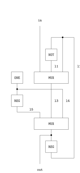
The devices making up this schematic will be modelled with predicates (Gordon 1986). For example, the predicate ONE is true of a signal out if for all times t the value of out is T.

> Definition ONE_def: ONE(out:num->bool) = !t. out t = T
  End
Definition has been stored under "ONE_def"
val ONE_def = ⊢ ∀out. ONE out ⇔ ∀t. out t ⇔ T: thm

Note that, as discussed above, 'ONE_def' is used both as an ML variable and as the name of the definition in the theory. Note also how ':num->bool' has been added to resolve type ambiguities; without this (or some other type information) the typechecker would not be able to infer that t is to have type num.

The binary predicate NOT is true of a pair of signals (inp,out) if the value of out is always the negation of the value of inp. Inverters are thus modelled as having no delay. This is appropriate for a register-transfer level model, but not at a lower level.

> Definition NOT_def:
     NOT(inp, out:num->bool) = !t. out t = ~(inp t)
  End
Definition has been stored under "NOT_def"
val NOT_def = ⊢ ∀inp out. NOT (inp,out) ⇔ ∀t. out t ⇔ ¬inp t: thm

The final combinational device needed is a multiplexer. This is a ‘hardware conditional’; the input sw selects which of the other two inputs are to be connected to the output out.

> Definition MUX_def:
    MUX(sw,in1,in2,out:num->bool) =
      !t. out t = if sw t then in1 t else in2 t
  End
Definition has been stored under "MUX_def"
val MUX_def =
   ⊢ ∀sw in1 in2 out.
       MUX (sw,in1,in2,out) ⇔ ∀t. out t ⇔ if sw t then in1 t else in2 t: thm

The remaining devices in the schematic are registers. These are unit-delay elements; the values output at time t+1 are the values input at the preceding time t, except at time 0 when the register outputs F.³

> Definition REG_def:
    REG(inp,out:num->bool) =
       !t. out t = if (t=0) then F else inp(t-1)
  End
Definition has been stored under "REG_def"
val REG_def =
   ⊢ ∀inp out. REG (inp,out) ⇔ ∀t. out t ⇔ if t = 0 then F else inp (t − 1):
   thm

The schematic diagram above can be represented as a predicate by conjoining the relations holding between the various signals and then existentially quantifying the internal lines. This technique is explained elsewhere (e.g. see (Camilleri, Melham, and Gordon 1987; Gordon 1986)).

> Definition PARITY_IMP_def:
    PARITY_IMP(inp,out) =
      ?l1 l2 l3 l4 l5.
        NOT(l2,l1) /\ MUX(inp,l1,l2,l3) /\ REG(out,l2) /\
        ONE l4     /\ REG(l4,l5)        /\ MUX(l5,l3,l4,out)
  End
Definition has been stored under "PARITY_IMP_def"
val PARITY_IMP_def =
   ⊢ ∀inp out.
       PARITY_IMP (inp,out) ⇔
       ∃l1 l2 l3 l4 l5.
         NOT (l2,l1) ∧ MUX (inp,l1,l2,l3) ∧ REG (out,l2) ∧ ONE l4 ∧
         REG (l4,l5) ∧ MUX (l5,l3,l4,out): thm

Verification

The following theorem will eventually be proved:

   |- !inp out. PARITY_IMP(inp,out) ==> (!t. out t = PARITY t inp)

This states that if inp and out are related as in the schematic diagram (i.e. as in the definition of PARITY_IMP), then the pair of signals (inp,out) satisfies the specification.

First, the following lemma is proved; the correctness of the parity checker follows from this and UNIQUENESS_LEMMA by the transitivity of ==>.

> g ‘!inp out.
       PARITY_IMP(inp,out) ==>
       (out 0 = T) /\
       !t. out(SUC t) = if inp(SUC t) then ~(out t) else out t’;
val it =
   Proof manager status: 2 proofs.
   2. Completed goalstack:
        ⊢ ∀inp out.
            (out 0 ⇔ T) ∧
            (∀t. out (SUC t) ⇔ if inp (SUC t) then ¬out t else out t) ⇒
            ∀t. out t ⇔ PARITY t inp
   
   1. Incomplete goalstack:
        Initial goal:
        ∀inp out.
          PARITY_IMP (inp,out) ⇒
          (out 0 ⇔ T) ∧
          ∀t. out (SUC t) ⇔ if inp (SUC t) then ¬out t else out t

The first step in proving this goal is to rewrite with definitions followed by a decomposition of the resulting goal using strip_tac. The rewriting tactic PURE_REWRITE_TAC is used; this does no built-in simplifications, only the ones explicitly given in the list of theorems supplied as an argument. One of the built-in simplifications used by REWRITE_TAC is |- ~(x = T) = x. PURE_REWRITE_TAC is used to prevent rewriting with this being done.

> e(PURE_REWRITE_TAC [PARITY_IMP_def, ONE_def, NOT_def,
                      MUX_def, REG_def] >>
    rpt strip_tac);
OK..
2 subgoals:
val it =
   
    0.  ∀t. l1 t ⇔ ¬l2 t
    1.  ∀t. l3 t ⇔ if inp t then l1 t else l2 t
    2.  ∀t. l2 t ⇔ if t = 0 then F else out (t − 1)
    3.  ∀t. l4 t ⇔ T
    4.  ∀t. l5 t ⇔ if t = 0 then F else l4 (t − 1)
    5.  ∀t. out t ⇔ if l5 t then l3 t else l4 t
   ------------------------------------
        out (SUC t) ⇔ if inp (SUC t) then ¬out t else out t
   
    0.  ∀t. l1 t ⇔ ¬l2 t
    1.  ∀t. l3 t ⇔ if inp t then l1 t else l2 t
    2.  ∀t. l2 t ⇔ if t = 0 then F else out (t − 1)
    3.  ∀t. l4 t ⇔ T
    4.  ∀t. l5 t ⇔ if t = 0 then F else l4 (t − 1)
    5.  ∀t. out t ⇔ if l5 t then l3 t else l4 t
   ------------------------------------
        out 0 ⇔ T

The top goal is the one printed last; its conclusion is out 0 = T and its assumptions are equations relating the values on the lines in the circuit. The natural next step would be to expand the top goal by rewriting with the assumptions. However, if this were done the system would go into an infinite loop because the equations for out, l2 and l3 are mutually recursive. Instead we use the first-order reasoner metis_tac to do the work:

> e(metis_tac []);
OK..
metis: r[+0+17]+0+0+0+0+0+1+0+1+0+1#

Goal proved.
 [......] ⊢ out 0 ⇔ T

Remaining subgoals:
val it =
   
    0.  ∀t. l1 t ⇔ ¬l2 t
    1.  ∀t. l3 t ⇔ if inp t then l1 t else l2 t
    2.  ∀t. l2 t ⇔ if t = 0 then F else out (t − 1)
    3.  ∀t. l4 t ⇔ T
    4.  ∀t. l5 t ⇔ if t = 0 then F else l4 (t − 1)
    5.  ∀t. out t ⇔ if l5 t then l3 t else l4 t
   ------------------------------------
        out (SUC t) ⇔ if inp (SUC t) then ¬out t else out t

The first of the two subgoals is proved. Inspecting the remaining goal it can be seen that it will be solved if its left hand side, out(SUC t), is expanded using the assumption:

   !t. out t = if l5 t then l3 t else l4 t

However, if this assumption is used for rewriting, then all the subterms of the form out t will also be expanded. To prevent this, we really want to rewrite with a formula that is specifically about out (SUC t). We want to somehow pull the assumption that we do have out of the list and rewrite with a specialised version of it. We can do just this using qpat_x_assum. This tactic is of type term quotation -> thm -> tactic. It selects an assumption that is of the form given by its first argument, and passes it to the second argument, a function which expects a theorem and returns a tactic. Here it is in action:

> e (qpat_x_assum ‘!t. out t = X t’
      (fn th => REWRITE_TAC [SPEC “SUC t” th]));
OK..
1 subgoal:
val it =
   
    0.  ∀t. l1 t ⇔ ¬l2 t
    1.  ∀t. l3 t ⇔ if inp t then l1 t else l2 t
    2.  ∀t. l2 t ⇔ if t = 0 then F else out (t − 1)
    3.  ∀t. l4 t ⇔ T
    4.  ∀t. l5 t ⇔ if t = 0 then F else l4 (t − 1)
   ------------------------------------
        (if l5 (SUC t) then l3 (SUC t) else l4 (SUC t)) ⇔
        if inp (SUC t) then ¬out t else out t

The pattern used here exploited something called higher order matching. The actual assumption that was taken off the assumption stack did not have a RHS that looked like the application of a function (X in the pattern) to the t parameter, but the RHS could nonetheless be seen as equal to the application of some function to the t parameter. In fact, the value that matched X was ``\x. if l5 x then l3 x else l4 x``.

Inspecting the goal above, it can be seen that the next step is to unwind the equations for the remaining lines of the circuit. We do using the standard simplifier rw.

> e (rw[]);
OK..   ... output elided ...

Goal proved.
 [......] ⊢ out (SUC t) ⇔ if inp (SUC t) then ¬out t else out t
val it =
   Initial goal proved.
   ⊢ ∀inp out.
       PARITY_IMP (inp,out) ⇒
       (out 0 ⇔ T) ∧ ∀t. out (SUC t) ⇔ if inp (SUC t) then ¬out t else out t

The theorem just proved is named PARITY_LEMMA and saved in the current theory.

> val PARITY_LEMMA = top_thm ();
val PARITY_LEMMA =
   ⊢ ∀inp out.
       PARITY_IMP (inp,out) ⇒
       (out 0 ⇔ T) ∧ ∀t. out (SUC t) ⇔ if inp (SUC t) then ¬out t else out t:
   thm

PARITY_LEMMA could have been proved in one step with a single compound tactic. Our initial goal can be expanded with a single tactic corresponding to the sequence of tactics that were used interactively:

> restart();   ... output elided ...
> e (PURE_REWRITE_TAC [PARITY_IMP_def, ONE_def, NOT_def,
                       MUX_def, REG_def] >>
    rpt strip_tac
    >- metis_tac []
    >- (qpat_x_assum ‘!t. out t = X t’
                 (fn th => REWRITE_TAC [SPEC “SUC t” th]) >>
        rw[]));
OK..
metis: r[+0+17]+0+0+0+0+0+1+0+1#
val it =
   Initial goal proved.
   ⊢ ∀inp out.
       PARITY_IMP (inp,out) ⇒
       (out 0 ⇔ T) ∧ ∀t. out (SUC t) ⇔ if inp (SUC t) then ¬out t else out t

Armed with PARITY_LEMMA, the final theorem is easily proved:

> Theorem PARITY_CORRECT:
    ∀inp out. PARITY_IMP(inp,out) ⇒ ∀t. out t = PARITY t inp
  Proof
    rpt strip_tac >> match_mp_tac UNIQUENESS_LEMMA >>
    irule PARITY_LEMMA >> rw[]
  QED
val PARITY_CORRECT =
   ⊢ ∀inp out. PARITY_IMP (inp,out) ⇒ ∀t. out t ⇔ PARITY t inp: thm

This completes the proof of the parity checking device.

Exercises

Two exercises are given in this section: Exercise 1 is straightforward, but Exercise 2 is quite tricky and might take a beginner several days to solve.

Exercise 1

Using only the devices ONE, NOT, MUX and REG defined in Section 5.3, design and verify a register RESET_REG with an input inp, reset line reset, output out and behaviour specified as follows.

• If reset is T at time t, then the value at out at time t is also T.
• If reset is T at time t or t+1, then the value output at out at time t+1 is T, otherwise it is equal to the value input at time t on inp.

This is formalized in HOL by the definition:

   RESET_REG(reset,inp,out) <=>
     (!t. reset t ==> (out t = T)) /\
     (!t. out(t+1) = if reset t \/ reset(t+1) then T else inp t)

Note that this specification is only partial; it doesn't specify the output at time 0 in the case that there is no reset.

The solution to the exercise should be a definition of a predicate RESET_REG_IMP as an existential quantification of a conjunction of applications of ONE, NOT, MUX and REG to suitable line names,⁴ together with a proof of:

   RESET_REG_IMP(reset,inp,out) ==> RESET_REG(reset,inp,out)

Exercise 2

1. Formally specify a resetable parity checker that has two boolean inputs reset and inp, and one boolean output out with the following behaviour:

   The value at out is T if and only if there have been an even number of Ts input at inp since the last time that T was input at reset.

2. Design an implementation of this specification built using only the devices ONE, NOT, MUX and REG defined in Section 5.3.

3. Verify the correctness of your implementation in HOL.

1. Signals are modelled as functions from numbers, representing times, to booleans. ↩

2. We'd like to use in as one of our variable names, but this is a reserved word for let-expressions. ↩

3. Time 0 represents when the device is switched on. ↩

4. i.e. a definition of the same form as that of PARITY_IMP on page \pageref{parity-imp}. ↩