Core Theories
The HOL system provides a collection of theories on which to base
verification tools or further theory development. In the rest of this
section, these theories are briefly described. The sections that
follow provide an overview of the contents of each theory. For a
complete list of all the axioms, definitions and theorems in HOL, see
the online resources distributed with the system. In particular, the
HTML file help/HOLindex.html is a good place to start browsing the
available theories. For a graphical picture of the theory hierarchy,
see help/theorygraph/theories.html.
In addition, core theories of higher mathematics are described in Chapter 6.
The Theory min
The starting theory of HOL is the theory min.
In this theory, the type constant bool of booleans, the binary type
operator $(\alpha,\beta)$fun of functions, and the type constant
ind of individuals are declared. Building on these types, three
primitive constants
are declared: equality, implication, and a choice operator:
- Equality
- Equality (
= : 'a -> 'a -> bool) is an infix operator. - Implication
- Implication (
==> : bool -> bool -> bool) is the material implication and is an infix operator that is right-associative, i.e.,x ==> y ==> zparses to the same term asx ==> (y ==> z). - Choice
- Equality and implication are standard predicate calculus notions,
but choice is more exotic: if $t$ is a term having type
$\sigma\to{}$
bool, then@x.$\,t\,$x(or, equivalently,$@$\,t$) denotes some member of the set whose characteristic function is $t$. If the set is empty, then@x.$\,t\,$xdenotes an arbitrary member of the set denoted by $\sigma$. The constant@is a higher order version of Hilbert's $\hilbert$-operator; it is related to the constant $\iota$ in Church's formulation of higher order logic. For more details, see Church's original paper (Church 1940), Leisenring's book on Hilbert's $\hilbert$-symbol (Leisenring 1969), or Andrews' textbook on type theory (Andrews 1986).
No theorems or axioms are placed in theory min. The primitive rules
of inference of HOL depend on the presence of min.
Basic Theories
The most basic theories in HOL provide support for a standard
collection of types. The theory bool defines the basis of the HOL
logic, including the boolean operations and quantifiers. On this
platform, quite a bit of theorem-proving infrastructure can already be
built. Further basic types are developed in the theory of pairs
(prod), disjoint sums (sum), the one-element type (one), and the
option type.
The theory bool
At start-up, the initial theory for users of the HOL system is called
bool, which is constructed when the HOL system is
built. The theory bool is an extension of the combination of the
“conceptual” theories LOG and INIT, described in the LOGIC manual.
Thus it contains the four axioms
for higher order logic. These axioms, together with the rules of
inference described in
Section 1.5.1,
constitute the core of the HOL logic. Because of the way the HOL
system evolved from LCF1, the
particular axiomatization of higher order logic it uses differs from
the classical axiomatization due to Church
(Church 1940). The biggest difference is that in Church's formulation
type variables
are in the meta-language, whereas in the HOL logic they are part of
the object language.
The logical constants
T (truth),
F (falsity),
~ (negation),
/\ (conjunction),
\/ (disjunction),
! (universal quantification),
? (existential quantification),
and ?! (unique existence quantifier)
can all be defined in terms of equality,
implication and choice. The definitions listed below are fairly
standard; each one is preceded by its ML name. Later definitions
sometimes build on earlier ones.
   T_DEF              |- T  = ((\x:bool. x) = (\x. x))

   FORALL_DEF         |- !  = \P:'a->bool. P = (\x. T)

   EXISTS_DEF         |- ?  = \P:'a->bool. P($@ P)

   AND_DEF            |- /\ = \t1 t2. !t. (t1 ==> t2 ==> t) ==> t

   OR_DEF             |- \/ = \t1 t2. !t. (t1 ==> t) ==> (t2 ==> t) ==> t

   F_DEF              |- F  = !t. t

   NOT_DEF            |- ~  = (\t. t ==> F)

   EXISTS_UNIQUE_DEF  |- ?! = (\P. $? P /\ (!x y. P x /\ P y ==> (x = y)))
There are four
axioms in the theory bool;
the first three are the following:
BOOL_CASES_AX
  ⊢ ∀t. (t ⇔ T) ∨ (t ⇔ F)

ETA_AX
  ⊢ ∀t. (λx. t x) = t

SELECT_AX
  ⊢ ∀P x. P x ⇒ P ($@ P)
The fourth and last axiom of the HOL logic is the Axiom of
Infinity. Its statement is phrased in terms
of the function properties ONE_ONE and ONTO. The definitions are:
ONE_ONE_DEF
  ⊢ ONE_ONE = (λf. ∀x1 x2. f x1 = f x2 ⇒ x1 = x2)
ONTO_DEF
  ⊢ ONTO = (λf. ∀y. ∃x. y = f x)
The Axiom of Infinity is
INFINITY_AX
  ⊢ ∃f. ONE_ONE f ∧ ¬ONTO f
This asserts that there exists a one-to-one map from ind to itself
that is not onto. This implies that the type ind denotes an
infinite set.
The three other axioms of the theory bool, the rules of inference in
Section 1.5.1
and the Axiom of Infinity are, together, sufficient for developing all
of standard mathematics. Thus, in principle, the user of the HOL
system should never need to make a non-definitional
theory. In practice, it is often very tempting to take the risk of
introducing new axioms because deriving them from definitions can be
tedious---proving that ‘axioms’ follow from definitions amounts to
proving their consistency.
Further definitions.
The theory bool also supplies the definitions of a number of useful
constants.
LET_DEF
  ⊢ LET = (λf x. f x)
COND_DEF
  ⊢ COND =
     (λt t1 t2. @x. ((t ⇔ T) ⇒ x = t1) ∧ ((t ⇔ F) ⇒ x = t2))
IN_DEF
  ⊢ $IN = (λx f. f x)
The constant LET
is used in representing terms containing local variable bindings
(i.e., let-terms).
For example, the concrete syntax let v = M in N is translated by the
parser to the term LET (\v.N) M. For the full description of how
let expressions are translated, see Section 5.2.3.2.
The constant COND is used to represent conditional expressions. The
concrete syntax
$\mathtt{if}\;t_1\;\mathtt{then}\;t_2\;\mathtt{else}\;t_3$ abbreviates
the application COND $t_1$ $t_2$ $t_3$.
The constant IN (written as an infix) is the basis of the modelling
of sets by their characteristic functions. The term $x$IN$P$ can
be read as "$x$ is an element of the set $P$", or (more in line with
its definition) as “the predicate $P$ is true of $x$”.
Finally, the polymorphic constant ARB$:\alpha$ denotes a fixed but
arbitrary element. ARB is occasionally useful when attempting to
deal with the issue of partiality.
Restricted quantifiers
The theory bool also defines constants that implement restricted
quantification. This provides a means of simulating subtypes and
dependent types with predicates. The most heavily used are
restrictions of the existential and universal quantifiers:
RES_FORALL_DEF
  ⊢ RES_FORALL = (λp m. ∀x. x ∈ p ⇒ m x)
RES_EXISTS_DEF
  ⊢ RES_EXISTS = (λp m. ∃x. x ∈ p ∧ m x)

RES_ABSTRACT_DEF
  ⊢ (∀p m x. x ∈ p ⇒ RES_ABSTRACT p m x = m x) ∧
     ∀p m1 m2.
       (∀x. x ∈ p ⇒ m1 x = m2 x) ⇒
       RES_ABSTRACT p m1 = RES_ABSTRACT p m2
The definition of RES_ABSTRACT is a characterising formula, rather
than a direct equation. There are two important properties
- if $y$ is an element of $P$ then $(\lambda x :: P.\; M)\,y = M[y/x]$
- if two restricted abstractions agree on all values over their (common) restricting set, then they are equal.
For completeness, restricted versions of unique existence and indefinite description are provided, although hardly used.
RES_EXISTS_UNIQUE_DEF
  ⊢ RES_EXISTS_UNIQUE =
     (λp m. (∃x::p. m x) ∧ ∀x y::p. m x ∧ m y ⇒ x = y)
RES_SELECT_DEF
  ⊢ RES_SELECT = (λp m. @x. x ∈ p ∧ m x)
The definition of RES_EXISTS_UNIQUE uses the restricted
quantification syntax with the :: symbol, referring to the earlier
definitions RES_EXISTS and RES_FORALL. The :: syntax is used
with restricted quantifiers to allow arbitrary predicates to restrict
binding variables. The HOL parser allows restricted quantification of
all of a sequence of binding variables by putting the restriction at
the end of the sequence, thus with a universal quantification:
$$ \forall x \, y \, z \, {\tt ::} \; P \, . \; Q(x,y,z) $$
Here the predicate $P$ restricts all of $x$, $y$ and $z$.
Derived syntactic forms
The HOL quotation parser
can translate various standard logical notations
into primitive terms. For example, if + has been declared an infix
(as explained in Section 1.6), as it is when
arithmeticTheory has been loaded, then x+1
is translated to “$+ x 1”. The escape character $
suppresses the infix behaviour of + and prevents the quotation
parser getting confused. In general, $ can be used to suppress any
special syntactic behaviour a token (such as if, + or let)
might have. This is illustrated in the table below, in which the
terms in the column headed ML quotation are translated by the
quotation parser to the corresponding terms in the column headed
Primitive term. Conversely, the terms in the latter column are
always printed in the form shown in the former one. The ML
constructor expressions in the rightmost column evaluate to the same
values (of type term) as the other quotations in the same row.
Table: Non-primitive terms
| Kind of term | ML quotation | Primitive term | Constructor expression |
|---|---|---|---|
| Negation | ~$t$ | $~ $t$ | mk_neg($t$) |
| Disjunction | $t_1$\/$t_2$ | $\/ $t_1\,t_2$ | mk_disj($t_1$,$t_2$) |
| Conjunction | $t_1$/\$t_2$ | $/\ $t_1\,t_2$ | mk_conj($t_1$,$t_2$) |
| Implication | $t_1$==>$t_2$ | $==> $t_1\,t_2$ | mk_imp($t_1$,$t_2$) |
| Equality | $t_1$=$t_2$ | $= $t_1\,t_2$ | mk_eq($t_1$,$t_2$) |
| $\forall$-quantification | !$x.t$ | $!(\$x.t$) | mk_forall($x$,$t$) |
| $\exists$-quantification | ?$x.t$ | $?(\$x.t$) | mk_exists($x$,$t$) |
| $\hilbert$-term | @$x.t$ | $@(\$x.t$) | mk_select($x$,$t$) |
| Conditional | if $t$then$t_1$else$t_2$ | COND $t\,t_1\,t_2$ | mk_cond($t$,$t_1$,$t_2$) |
let-expression | let $x$=$t_1$in$t_2$ | LET(\$x.t_2$)$t_1$ | mk_let(mk_abs($x$,$t_2$),$t_1$) |
There are constructors, destructors and indicators for all the obvious
constructs. (Indicators, e.g., is_neg, return truth values
indicating whether or not a term belongs to the syntax class in
question.) In addition to the constructors listed in the table there
are constructors, destructors, and indicators for pairs and lists,
namely mk_pair,
mk_cons
and mk_list
(see the REFERENCE manual). The constants COND and LET are
explained in the section on
The theory bool above. The constants \/,
/\, ==> and = are examples of infixes and represent $\vee$,
$\wedge$, $\Rightarrow$ and equality, respectively. If $c$ is
declared to be an infix, then the HOL parser will translate
$t_1\;c\;t_2$ to $\mathtt{\$}c;t_1;t_2$.
The constants !, ? and @ are examples of
*binders*
and represent $\forall$, $\exists$ and $\hilbert$, respectively. If
$c$ is declared to be a binder, then the HOL parser will translate
$c;x.t$ to the combination $\mathtt{$}c\,(\lambda x.\,t)$ (i.e., the
application of the constant $c$ to the representation of the
abstraction $\lambda x.\,t$).
Table: Syntactic abbreviations
| Abbreviated term | Meaning | Constructor expression |
|---|---|---|
| $t\,t_1\cdots t_n$ | ($\cdots$($t\,t_1$)$\cdots t_n$) | list_mk_comb($t$,[$t_1$, $\ldots$ ,$t_n$]) |
\$x_1\cdots x_n$.$t$ | \$x_1$. $\cdots$ \$x_n$.$t$ | list_mk_abs([$x_1$, $\ldots$ ,$x_n$],$t$) |
!$x_1\cdots x_n$.$t$ | !$x_1$. $\cdots$ !$x_n$.$t$ | list_mk_forall([$x_1$, $\ldots$ ,$x_n$],$t$) |
?$x_1\cdots x_n$.$t$ | ?$x_1$. $\cdots$ ?$x_n$.$t$ | list_mk_exists([$x_1$, $\ldots$ ,$x_n$],$t$) |
There are also constructors
list_mk_conj,
list_mk_disj,
list_mk_imp
for conjunctions, disjunctions, and implications respectively. The
corresponding destructor functions are called strip_comb etc.
Theorems
A large number of theorems involving the logical constants are
pre-proved in the theory bool. The following theorems illustrate
how higher order logic allows concise expression of theorems
supporting quantifier movement.
 LEFT_AND_FORALL_THM  |- !P Q. (!x. P x) /\ Q = !x. P x /\ Q
 RIGHT_AND_FORALL_THM |- !P Q. P /\ (!x. Q x) = !x. P /\ Q x

 LEFT_EXISTS_AND_THM  |- !P Q. (?x. P x /\ Q) = (?x. P x) /\ Q
 RIGHT_EXISTS_AND_THM |- !P Q. (?x. P /\ Q x) = P /\ ?x. Q x

 LEFT_FORALL_IMP_THM  |- !P Q. (!x. P x ==> Q) = (?x. P x) ==> Q
 RIGHT_FORALL_IMP_THM |- !P Q. (!x. P ==> Q x) = P ==> !x. Q x

 LEFT_EXISTS_IMP_THM  |- !P Q. (?x. P x ==> Q) = (!x. P x) ==> Q
 RIGHT_EXISTS_IMP_THM |- !P Q. (?x. P ==> Q x) = P ==> ?x. Q x

 LEFT_FORALL_OR_THM   |- !Q P. (!x. P x \/ Q) = (!x. P x) \/ Q
 RIGHT_FORALL_OR_THM  |- !P Q. (!x. P \/ Q x) = P \/ !x. Q x

 LEFT_OR_EXISTS_THM   |- !P Q. (?x. P x) \/ Q = ?x. P x \/ Q
 RIGHT_OR_EXISTS_THM  |- !P Q. P \/ (?x. Q x) = ?x. P \/ Q x

 EXISTS_OR_THM        |- !P Q. (?x. P x \/ Q x) = (?x. P x) \/ ?x. Q x
 FORALL_AND_THM       |- !P Q. (!x. P x /\ Q x) = (!x. P x) /\ !x. Q x

 NOT_EXISTS_THM       |- !P. ~(?x. P x) = !x. ~P x
 NOT_FORALL_THM       |- !P. ~(!x. P x) = ?x. ~P x

 SKOLEM_THM           |- !P. (!x. ?y. P x y) = ?f. !x. P x (f x)
Also, a theorem justifying Skolemization (SKOLEM_THM) is proved.
Many other theorems may be found in bool theory.
Combinators
The theory combin
contains the definitions of function composition (infixed o),
a reversed function application operator,
function override (infixed =+),
and the combinators S,
K,
I,
W,
and C.
o_DEF
  ⊢ ∀f g. f ∘ g = (λx. f (g x))
APP_DEF
  ⊢ ∀x f. (x :> f) = f x
UPDATE_def
  ⊢ ∀a b. (a =+ b) = (λf c. if a = c then b else f c)
K_DEF
  ⊢ K = (λx y. x)
S_DEF
  ⊢ S = (λf g x. f x (g x))
I_DEF
  ⊢ I = S K K
W_DEF
  ⊢ W = (λf x. f x x)
C_DEF
  ⊢ flip = (λf x y. f y x)
The following elementary properties are proved in the theory combin:
o_THM
  ⊢ ∀f g x. (f ∘ g) x = f (g x)
o_ASSOC
  ⊢ ∀f g h. f ∘ g ∘ h = (f ∘ g) ∘ h

UPDATE_EQ
  ⊢ ∀f a b c. f⦇a ↦ c; a ↦ b⦈ = f⦇a ↦ c⦈
UPDATE_COMMUTES
  ⊢ ∀f a b c d. a ≠ b ⇒ f⦇a ↦ c; b ↦ d⦈ = f⦇b ↦ d; a ↦ c⦈
APPLY_UPDATE_THM
  ⊢ ∀f a b c. f⦇a ↦ b⦈ c = if a = c then b else f c

K_THM
  ⊢ ∀x y. K x y = x
S_THM
  ⊢ ∀f g x. S f g x = f x (g x)
I_THM
  ⊢ ∀x. I x = x
W_THM
  ⊢ ∀f x. W f x = f x x
C_THM
  ⊢ ∀f x y. flip f x y = f y x
The above illustrates that there are two ways of writing function
update terms. As per the definition above (UPDATE_def), the infix
=+ takes a key $k$ and a value $v$, and returns a higher-order
function, which when in turn is passed a function $f$, returns a
version of that function that has been updated to return $v$ when
applied to $k$, and is otherwise the same as $f$. The same effect
can be achieved with the “substitution style” syntax:
$f\llparenthesis k\mapsto v\rrparenthesis$. There is an ASCII form
of this notation as well:
> ``(k2 =+ v2) ((k1 =+ v1) f)``;
<<HOL message: inventing new type variable names: 'a, 'b>>
val it = “f⦇k2 ↦ v2; k1 ↦ v1⦈”: term
> ``f (| k |-> v |)``;
<<HOL message: inventing new type variable names: 'a, 'b>>
val it = “f⦇k ↦ v⦈”: term
There are no theorems about :>; its use is as a convenient syntax
for function applications. For example, chains of updates can lose
some parentheses if written
f :> (k1 =+ v1) :> (k2 =+ v2) :> (k3 =+ v3)
This presentation also makes the order in which functions are applied read from left-to-right.
Having the symbols o, S, K, I, W, and C as built-in
constants
is sometimes inconvenient because they are often wanted as mnemonic
names for variables (e.g., S to range over sets and o to range
over outputs).2 Variables with these names can be
used in the current system if o, S, K, I, W, and C are
first hidden (see Section 8.1.2.8). In fact, this happens so
often with the constant C that the name C is “hidden” by
default.
Instead, it can be written in fully-qualified form, as combin$C,
or with the alias flip, as can be seen above.
Pairs
The Cartesian product type operator
prod
is defined in the theory pair. Values of type
($\sigma_1$,$\sigma_2$)prod are ordered pairs whose first
component has type $\sigma_1$ and whose second component has type
$\sigma_2$. The HOL type parser
converts type expressions of the form :$\sigma_1$#$\sigma_2$
into ($\sigma_1$,$\sigma_2$)prod,
and the printer inverts this transformation. Pairs
are constructed with an infixed comma symbol
$, : 'a -> 'b -> 'a # 'b
so, for example, if $t_1$ and $t_2$ have types $\sigma_1$ and
$\sigma_2$ respectively, then $t_1$,$t_2$ is a term with type
$\sigma_1$#$\sigma_2$. Usually, pairs are written within
brackets: ($t_1$,$t_2$). The comma symbol associates
to the right, so that ($t_1$,$t_2$,$\ldots$,$t_n$) means
($t_1$,($t_2$,$\ldots$,$t_n$)).
Defining the product type.
The type of Cartesian products is defined by representing a pair
($t_1$,$t_2$) by the function
\a b. (a = t1) /\ (b = t2)
The representing type of $\sigma_1$#$\sigma_2$ is thus
$\sigma_1$->$\sigma_2$->bool. It is easy to prove the following
theorem.3
|- ?p:'a->'b->bool. (\p. ?x y. p = \a b. (a = x) /\ (b = y)) p
The type operator prod is defined by invoking
new_type_definition
with this theorem which results in the definitional axiom
prod_TY_DEF shown below being asserted in the theory pair.
prod_TY_DEF
  ⊢ ∃rep.
       TYPE_DEFINITION (λp. ∃x y. p = (λa b. a = x ∧ b = y)) rep
Next, the representation and abstraction functions REP_prod and
ABS_prod for the new type are introduced, along with the following
characterizing theorem, by use of the function
define_new_type_bijections.
ABS_REP_prod
  ⊢ (∀a. ABS_prod (REP_prod a) = a) ∧
     ∀r. (λp. ∃x y. p = (λa b. a = x ∧ b = y)) r ⇔
         REP_prod (ABS_prod r) = r
Pairs and projections.
The infix constructor ',' is then defined to be an application of
the abstraction function. Subsequently, two crucial theorems are
proved: PAIR_EQ asserts that equal pairs have equal components and
ABS_PAIR_THM shows that every term having a product type can be
decomposed into a pair of terms.
COMMA_DEF
  ⊢ ∀x y. (x,y) = ABS_prod (λa b. a = x ∧ b = y)
PAIR_EQ
  ⊢ (x,y) = (a,b) ⇔ x = a ∧ y = b
ABS_PAIR_THM
  ⊢ ∀x. ∃q r. x = (q,r)
By Skolemizing ABS_PAIR_THM and making constant specifications for
FST and SND, the following theorems are proved.
PAIR
  ⊢ ∀x. (FST x,SND x) = x
FST
  ⊢ ∀x y. FST (x,y) = x
SND
  ⊢ ∀x y. SND (x,y) = y
Pairs and functions.
In HOL, a function of type $\alpha\#\beta\to\gamma$ always has a
counterpart of type $\alpha\to\beta\to\gamma$, and vice versa.
This conversion is accomplished by the functions CURRY and
UNCURRY. These functions are inverses.
CURRY_DEF
  ⊢ ∀f x y. CURRY f x y = f (x,y)
UNCURRY_DEF
  ⊢ ∀f x y. UNCURRY f (x,y) = f x y

CURRY_UNCURRY_THM
  ⊢ ∀f. CURRY (UNCURRY f) = f
UNCURRY_CURRY_THM
  ⊢ ∀f. UNCURRY (CURRY f) = f
Mapping functions over a pair.
Functions $f:\alpha\to\gamma_1$ and $g:\beta\to\gamma_2$ can be
applied component-wise (##, infix) over a pair of type
$\alpha\#\beta$ to obtain a pair of type $\gamma_1\#\gamma_2$.
PAIR_MAP_THM
  ⊢ ∀f g x y. (f ## g) (x,y) = (f x,g y)
Binders and pairs. When doing proofs, statements involving tuples may take the form of a binding (quantification or $\lambda$-abstraction) of a variable with a product type. It may be convenient in subsequent reasoning steps to replace the variables with tuples of variables. The following theorems support this.
FORALL_PROD
  ⊢ (∀p. P p) ⇔ ∀p_1 p_2. P (p_1,p_2)
EXISTS_PROD
  ⊢ (∃p. P p) ⇔ ∃p_1 p_2. P (p_1,p_2)
LAMBDA_PROD
  ⊢ ∀P. (λp. P p) = (λ(p1,p2). P (p1,p2))
The theorem LAMBDA_PROD involves a paired abstraction, discussed
in Section 5.2.3.1.
Wellfounded relations on pairs.
Wellfoundedness, defined in Section 5.3.1.4, is a
useful notion, especially for proving termination of recursive
functions. For pairs, the lexicographic combination of relations
(LEX, infix) may be defined by using paired abstractions. Then
the theorem that lexicographic combination of wellfounded relations
delivers a wellfounded relation is easy to prove.
LEX_DEF
  ⊢ ∀R1 R2. R1 LEX R2 = (λ(s,t) (u,v). R1 s u ∨ s = u ∧ R2 t v)
WF_LEX
  ⊢ ∀R Q. WF R ∧ WF Q ⇒ WF (R LEX Q)
Paired abstractions
It is notationally convenient to include pairing in the lambda
notation, as a simple pattern-matching mechanism. The quotation
parser
will convert the term \($x_1$,$x_2$).$t$ to
UNCURRY(\$x_1\,x_2$.$t$). The transformation is done
recursively so that, for example,
\(x1, x2, x3). t
is converted to
UNCURRY (\x1. UNCURRY(\x2 x3. t))
More generally, the quotation parser repeatedly applies the transformation:
$$ \mathtt{\backslash(}v_1\mathtt{,}v_2\mathtt{).}t \quad\leadsto\quad \mathtt{UNCURRY(\backslash}v_1\mathtt{.\backslash}v_2\mathtt{.}t\mathtt{)} $$
until no more variable structures remain. For example:
$$ \begin{aligned} \mathtt{\backslash(}x\mathtt{,}y\mathtt{).}t &\;\leadsto\; \mathtt{UNCURRY(\backslash}x\,y\mathtt{.}t\mathtt{)}\\ \mathtt{\backslash(}x_1\mathtt{,}x_2\mathtt{,}\ldots\mathtt{,}x_n\mathtt{).}t &\;\leadsto\; \mathtt{UNCURRY(\backslash}x_1\mathtt{.\backslash(}x_2\mathtt{,}\ldots\mathtt{,}x_n\mathtt{).}t\mathtt{)}\\ \mathtt{\backslash((}x_1\mathtt{,}\ldots\mathtt{,}x_n\mathtt{),}y_1\mathtt{,}\ldots\mathtt{,}y_m\mathtt{).}t &\;\leadsto\; \mathtt{UNCURRY(\backslash(}x_1\mathtt{,}\ldots\mathtt{,}x_n\mathtt{).\backslash(}y_1\mathtt{,}\ldots\mathtt{,}y_m\mathtt{).}t\mathtt{)} \end{aligned} $$
As a result of this parser translation, a variable structure, such
as (x,y) in \(x,y).x+y, is not a subterm of the abstraction
in which it occurs; it disappears on parsing.
This can lead to unexpected errors (accompanied by obscure error
messages). For example, antiquoting a pair into the bound variable
position of a lambda abstraction fails:
> ``\(x,y).x+y``;
val it = “λ(x,y). x + y”: term

> val p = Term `(x:num,y:num)`;
val p = “(x,y)”: term

> Lib.try Term `\^p.x+y` handle _ => T

Exception raised at Term.dest_var: not a var
val it = “T”: term
If $b$ is a binder, then `b(x_1,x_2).t` is parsed as
`b(\(x_1,x_2).t)`, and hence transformed as above. For
example, !(x,y). x > y parses to $!(UNCURRY(\x.\y. x > y)).
let-terms
The quotation parser
accepts let-terms
similar to those in ML. For example, the following terms are
allowed:
   let x = 1 and y = 2 in x+y

   let f(x,y) = (x*x)+(y*y); a = 20*20; b = 50*49 in f(a,b)
let-terms are actually abbreviations for ordinary terms which are
specially supported by the parser and pretty printer. The constant
LET
is defined (in the theory bool) by:
LET = (\f x. f x)
and is used to encode let-terms in the logic. The parser
repeatedly applies the transformations:
$$ \begin{aligned} \mathtt{let}\ f\,v_1\,\ldots\,v_n=t_1\ \mathtt{in}\ t_2 &\;\leadsto\; \mathtt{LET(\backslash} f\mathtt{.}t_2\mathtt{)(\backslash} v_1\,\ldots\,v_n\mathtt{.}t_1\mathtt{)}\\ \mathtt{let}\ (v_1,\ldots,v_n)=t_1\ \mathtt{in}\ t_2 &\;\leadsto\; \mathtt{LET(\backslash(}v_1\mathtt{,}\ldots\mathtt{,}v_n\mathtt{).}t_2\mathtt{)}t_1\\ \mathtt{let}\ v_1=t_1\,\mathtt{and}\,\ldots\,\mathtt{and}\,v_n=t_n\ \mathtt{in}\ t &\;\leadsto\; \mathtt{LET(\ldots(LET(LET(\backslash}v_1\ldots v_n\mathtt{.} t\mathtt{)}t_1\mathtt{)}t_2\mathtt{)\ldots)}t_n \end{aligned} $$
The underlying structure of the term can be seen by applying destructor operations. For example:
> Term `let x = 1; y = 2; in x+y`;
val it = “let x = 1; y = 2 in x + y”: term

> dest_comb it;
val it = (“LET (λx. (let y = 2 in x + y))”, “1”): term * term

> Term `let (x,y) = (1,2) in x+y`;
val it = “let (x,y) = (1,2) in x + y”: term

> dest_comb it;
val it = (“LET (λ(x,y). x + y)”, “(1,2)”): term * term
Readers are encouraged to convince themselves that the translations
of let-terms represent the intuitive meaning suggested by the
surface syntax.
Disjoint sums
The theory sum defines the binary disjoint union type operator
sum. A type ($\sigma_1$,$\sigma_2$)sum denotes the disjoint
union of types $\sigma_1$ and $\sigma_2$. The type operator sum
can be defined, just as prod was, but the details are omitted
here.4 The HOL parser
converts :$\sigma_1$+$\sigma_2$`` `` into `` ``:($\sigma_1$,$\sigma_2$`)sum , and the printer
inverts this.
The standard operations on sums are:
   INL  : 'a -> 'a + 'b
   INR  : 'b -> 'a + 'b
   ISL  : 'a + 'b -> bool
   ISR  : 'a + 'b -> bool
   OUTL : 'a + 'b -> 'a
   OUTR : 'a + 'b -> 'b
These are all defined as constants in the theory sum. The
constants INL and INR inject into the left and right summands,
respectively. The constants ISL and ISR test for membership of
the left and right summands, respectively. The constants OUTL and
OUTR project from a sum to the left and right summands,
respectively.
The following theorem is proved in the theory sum. It provides a
complete and abstract characterization of the disjoint sum type, and
is used to justify the definition of functions over sums.
sum_Axiom
  ⊢ ∀f g. ∃h. (∀x. h (INL x) = f x) ∧ ∀y. h (INR y) = g y
Also provided are the following theorems having to do with the
discriminator functions ISL and ISR:
ISL
  ⊢ (∀x. ISL (INL x) ⇔ T) ∧ ∀y. ISL (INR y) ⇔ F
ISR
  ⊢ (∀x. ISR (INR x) ⇔ T) ∧ ∀y. ISR (INL y) ⇔ F

ISL_OR_ISR
  ⊢ ∀x. ISL x ∨ ISR x
The sum theory also provides the following theorems relating the
projection functions and the discriminators.
OUTL
  ⊢ ∀x. OUTL (INL x) = x
OUTR
  ⊢ ∀x. OUTR (INR x) = x

INL
  ⊢ ∀x. ISL x ⇒ INL (OUTL x) = x
INR
  ⊢ ∀x. ISR x ⇒ INR (OUTR x) = x
The sum type operator can be seen as functorial over its arguments
and so has a “map” function, SUM_MAP, with definition and results
showing its functoriality:
SUM_MAP_def
  ⊢ (∀f g a. SUM_MAP f g (INL a) = INL (f a)) ∧
     ∀f g b. SUM_MAP f g (INR b) = INR (g b)
SUM_MAP_I
  ⊢ SUM_MAP I I = I
SUM_MAP_o
  ⊢ SUM_MAP f g ∘ SUM_MAP h k = SUM_MAP (f ∘ h) (g ∘ k)
The one-element type
The theory one defines the type one which contains one element.
The type is also abbreviated as unit, which is the name of the
analogous type in ML, and this is the type's preferred printing
form. The constant one denotes this one element, but, again by
analogy with ML, the preferred parsing and printing form for this
constant is ().5 The pre-proved theorems in the
theory one are:
one_axiom
  ⊢ ∀(f :α -> unit) (g :α -> unit). f = g
one
  ⊢ ∀(v :unit). v = ()
one_Axiom
  ⊢ ∀(e :α). ∃!(fn :unit -> α). fn () = e
These three theorems are equivalent characterizations of the type
with only one value. The theory one is typically used in
constructing more elaborate types.
The itself type
The unary itself type operator (in boolTheory) provides a family
of singleton types akin to one. Thus, for every type $\alpha$,
`α itself` is a type containing just one value. This value's
name is the_value, but the parser and pretty-printer are set up so
that for the type `α itself`, the_value can be written as
`(:α)` (the syntax includes the parentheses). For example,
(:num) is the single value inhabiting the type num itself.
The point of the itself type is that if one defines a function with
`α itself` as the domain, the function picks out just one
value in its range, and so one can think of the function as being
one from the type to a value for the whole type.
For example, one could define
finite_univ (:'a) = FINITE (UNIV :'a set)
It would then be straightforward to prove the following theorems
   ⊢ finite_univ(:bool)
   ⊢ ¬finite_univ(:num)
   ⊢ finite_univ(:'a) ∧ finite_univ(:'b) ⇒ finite_univ(:'a # 'b)
The itself type is used in the Finite Cartesian Product construction that underlies the fixed-width word type (see Section 5.3.8 below).
The option type
The theory option defines a type operator option that ‘lifts’
its argument type, creating a type with all of the values of the
argument and one other, specially distinguished value. The
constructors of this type are
   NONE : 'a option
   SOME : 'a -> 'a option
Options can be used to model partial functions. If a function of
type $\alpha\rightarrow\beta$ does not have useful $\beta$ values
for all $\alpha$ inputs, then this distinction can be marked by
making the range of the function $\beta\,$option, and mapping the
undefined $\alpha$ values to NONE.
An inductive type, options have a recursion theorem supporting the definition of primitive recursive functions over option values.
option_Axiom
  ⊢ ∀e f. ∃fn. fn NONE = e ∧ ∀x. fn (SOME x) = f x
The option theory also defines a case constant that allows one to
inspect option values in a “pattern-matching” style.
   case e of
     NONE => u
   | SOME x => f x
The constant underlying this syntactic sugar is option_CASE with
definition
option_case_def
  ⊢ (∀v f. option_CASE NONE v f = v) ∧
     ∀x v f. option_CASE (SOME x) v f = f x
Another useful function maps a function over an option:
OPTION_MAP_DEF
  ⊢ (∀f x. OPTION_MAP f (SOME x) = SOME (f x)) ∧
     ∀f. OPTION_MAP f NONE = NONE
Finally, the THE function takes a SOME value to that
constructor's argument, and is unspecified on NONE:
THE_DEF
  ⊢ ∀x. THE (SOME x) = x
Numbers
The natural numbers, integers, and real numbers are provided in a series of theories. Also available are theories of extended real numbers, $n$-bit words (numbers modulo $2^n$), floating point and fixed point numbers.
Natural numbers
The natural numbers are developed in a series of theories: num,
prim_rec, arithmetic, and numeral. In num, the type of
numbers is defined from the Axiom of Infinity, and Peano's axioms
are derived. In prim_rec the Primitive Recursion theorem is
proved. Based on that, a large theory treating the standard
arithmetic operations is developed in arithmetic. Lastly, a
theory of numerals is developed in numeral.
The theory num
The theory num
defines the type num of natural numbers to be isomorphic to a
countable subset of the primitive type ind. In this theory, the
constants 0
and SUC (the successor function) are defined and Peano's axioms
pre-proved in the form:
NOT_SUC
  ⊢ ∀n. SUC n ≠ 0
INV_SUC
  ⊢ ∀m n. SUC m = SUC n ⇒ m = n
INDUCTION
  ⊢ ∀P. P 0 ∧ (∀n. P n ⇒ P (SUC n)) ⇒ ∀n. P n
In higher order logic, Peano's axioms are sufficient for developing
number theory because addition and multiplication can be defined.
In first order logic these must be taken as primitive. Note also
that INDUCTION could not be stated as a single axiom in first
order logic because predicates (e.g., P) cannot be quantified.
The theory prim_rec
In classical logic, unlike domain theory logics such as PP$\lambda$,
arbitrary recursive definitions
are not allowed. For example, there is no function $f$ (of type
num->num) such that
!x. f x = (f x) + 1
Certain restricted forms of recursive
definition do, however, uniquely define functions. An important
example are the primitive recursive functions.6
For any $x$ and $f$ the primitive recursion theorem tells us that
there is a unique function fn such that:
(fn 0 = x) /\ (!n. fn(SUC n) = f (fn n) n)
The primitive recursion theorem, named num_Axiom in HOL, follows
from Peano's
axioms.
num_Axiom
  ⊢ ∀e f. ∃fn. fn 0 = e ∧ ∀n. fn (SUC n) = f n (fn n)
The theorem states the validity of primitive recursive definitions
on the natural numbers: for any x and f there exists a
corresponding total function fn which satisfies the primitive
recursive definition whose form is determined by x and f.
The less-than relation.
The less-than relation '<'
is most naturally defined by primitive recursion. However, in our
development it is needed for the proof of the primitive recursion
theorem, so it must be defined before definition by primitive
recursion is available. The theory prim_rec therefore contains
the following non-recursive definition of <:
LESS_DEF
  ⊢ ∀m n. m < n ⇔ ∃P. (∀n. P (SUC n) ⇒ P n) ∧ P m ∧ ¬P n
This definition says that m < n if there exists a set (with
characteristic function P) that is downward
closed7 and contains m but not n.
Mechanizing primitive recursive definitions
The primitive recursion theorem can be used to justify any definition of a function on the natural numbers by primitive recursion. For example, a primitive recursive definition in higher order logic of the form
$$ \begin{aligned} \mathtt{fun}\,0\,x_1\,\ldots\,x_i &= f_1[x_1,\ldots,x_i]\\ \mathtt{fun}\,(\mathtt{SUC}\,n)\,x_1\,\ldots\,x_i &= f_2[\mathtt{fun}\,n\,t_1\,\ldots\,t_i,\,n,\,x_1,\ldots,x_i] \end{aligned} $$
where all the free variables in the terms $t_1,\ldots,t_i$ are contained in $\{n,x_1,\ldots,x_i\}$, is logically equivalent to:
$$ \begin{aligned} \mathtt{fun}\,0 &= \lambda x_1\,\ldots\,x_i.\,f_1[x_1,\ldots,x_i]\\ \mathtt{fun}\,(\mathtt{SUC}\,n) &= \lambda x_1\,\ldots\,x_i.\,f_2[\mathtt{fun}\,n\,t_1\,\ldots\,t_i,\,n,\,x_1,\ldots,x_i]\\ &= (\lambda f\,n\,x_1\,\ldots\,x_i.\,f_2[f\,t_1\,\ldots\,t_i,\,n,\,x_1,\ldots,x_i])\,(\mathtt{fun}\,n)\,n \end{aligned} $$
The existence of a recursive function fun which satisfies these
two equations follows directly from the primitive recursion theorem
num_Axiom shown above. Specializing the quantified variables x
and f in a suitably type-instantiated version of num_Axiom so
that
$$ \begin{aligned} x &= \lambda x_1\,\ldots\,x_i.\,f_1[x_1,\ldots,x_i]\quad\text{and}\\ f &= \lambda f\,n\,x_1\,\ldots\,x_i.\,f_2[f\,t_1\,\ldots\,t_i,\,n,\,x_1,\ldots,x_i] \end{aligned} $$
yields the existence theorem shown below:
$$ \begin{aligned} \vdash\,\exists\mathtt{fn}.\, &\mathtt{fn}\,0 = \lambda x_1\,\ldots\,x_i.\,f_1[x_1,\ldots,x_i]\;\wedge\\ &\mathtt{fn}\,(\mathtt{SUC}\,n) = (\lambda f\,n\,x_1\,\ldots\,x_i.\,f_2[f\,t_1\,\ldots\,t_i,\,n,\,x_1,\ldots,x_i])\,(\mathtt{fn}\,n)\,n \end{aligned} $$
This theorem allows a constant fun to be introduced (via the
definitional mechanism of constant specifications—see Section
1.6.3.2) to denote the recursive function that satisfies the
two equations in the body of the theorem. Introducing a constant
fun to name the function asserted to exist by the theorem shown
above, and simplifying using $\beta$-reduction, yields the
following theorem:
$$ \begin{aligned} \vdash\, &\mathtt{fun}\,0 = \lambda x_1\,\ldots\,x_i.\,f_1[x_1,\ldots,x_i]\;\wedge\\ &\mathtt{fun}\,(\mathtt{SUC}\,n) = \lambda x_1\,\ldots\,x_i.\,f_2[\mathtt{fun}\,n\,t_1\,\ldots\,t_i,\,n,\,x_1,\ldots,x_i] \end{aligned} $$
It follows immediately from this theorem that the constant fun
satisfies the primitive recursive defining equations given by the
theorem shown below:
$$ \begin{aligned} \vdash\, &\mathtt{fun}\,0\,x_1\,\ldots\,x_i = f_1[x_1,\ldots,x_i]\\ &\mathtt{fun}\,(\mathtt{SUC}\,n)\,x_1\,\ldots\,x_i = f_2[\mathtt{fun}\,n\,t_1\,\ldots\,t_i,\,n,\,x_1,\ldots,x_i] \end{aligned} $$
To automate the use of the primitive recursion theorem in deriving recursive definitions of this kind, the HOL system provides a function which automatically proves the existence of primitive recursive functions and then makes a constant specification to introduce the constant that denotes such a function:
   new_recursive_definition :
      {def : term, name : string, rec_axiom : thm} -> thm
In fact, new_recursive_definition handles primitive recursive
definitions over a range of types, not just the natural numbers.
For details, see the REFERENCE documentation.
More conveniently still, the Define function (see Section
8.3.1) supports primitive recursion,
along with other styles of recursion, and does not require the user
to quote the primitive recursion axiom. It may, however, require
termination proofs to be performed; fortunately, these need not be
done for primitive recursions.
Dependent choice and wellfoundedness
The primitive recursion theorem is useful beyond its main purpose
of justifying recursive definitions. For example, the theory
prim_rec proves the Axiom of Dependent Choice (DC).
DC
  ⊢ ∀P R a.
       P a ∧ (∀x. P x ⇒ ∃y. P y ∧ R x y) ⇒
       ∃f. f 0 = a ∧ ∀n. P (f n) ∧ R (f n) (f (SUC n))
The proof uses SELECT_AX. The theorem DC is useful when one
wishes to build a function having a certain property from a
relation. For example, one way to define the wellfoundedness of a
relation $R$ is to say that it has no infinite decreasing $R$
chains.
wellfounded_def
  ⊢ ∀R. Wellfounded R ⇔ ¬∃f. ∀n. R (f (SUC n)) (f n)
WF_IFF_WELLFOUNDED
  ⊢ ∀R. WF R ⇔ Wellfounded R
By use of DC, this statement can be proved to be equal to the
notion of wellfoundedness WF (namely, that every set has an
$R$-minimal element) defined in the theory relation.
Theorems asserting the wellfoundedness of the predecessor relation
and the less-than relation, as well as the wellfoundedness of
measure functions are also proved in prim_rec.
WF_PRED
  ⊢ WF (λx y. y = SUC x)
WF_LESS
  ⊢ WF $<

measure_def
  ⊢ measure = inv_image $<
measure_thm
  ⊢ ∀f x y. measure f x y ⇔ f x < f y
WF_measure
  ⊢ ∀m. WF (measure m)
Arithmetic
The HOL theory arithmetic contains primitive recursive definitions
of the following standard arithmetic operators.
ADD
  ⊢ (∀n. 0 + n = n) ∧ ∀m n. SUC m + n = SUC (m + n)

SUB
  ⊢ (∀m. 0 − m = 0) ∧
     ∀m n. SUC m − n = if m < n then 0 else SUC (m − n)

MULT
  ⊢ (∀n. 0 * n = 0) ∧ ∀m n. SUC m * n = m * n + n

EXP
  ⊢ (∀m. m ** 0 = 1) ∧ ∀m n. m ** SUC n = m * m ** n
Note that EXP is an infix. The infix notation ** may be used
in place of EXP. Thus (x EXP y) means $x^y$, and so does
(x ** y). In addition, the parser special-cases superscript 2
and 3 notations, so that `x²` is actually the same term as
x EXP 2, and `x³` is the same term as x EXP 3.
Comparison operators.
A full set of comparison operators is defined in terms of <.
GREATER_DEF
  ⊢ ∀m n. m > n ⇔ n < m
LESS_OR_EQ
  ⊢ ∀m n. m ≤ n ⇔ m < n ∨ m = n
GREATER_OR_EQ
  ⊢ ∀m n. m ≥ n ⇔ m > n ∨ m = n
Note that in all of HOL's standard numeric theories, it is usual practice to avoid uses of the “greater-than” constants and to express everything with either $<$ or $\le$.
Division and modulus.
A constant specification is used to introduce division (DIV,
infix) and modulus (MOD, infix) operators, together with their
characterizing property.
DIVISION
  ⊢ ∀n. 0 < n ⇒ ∀k. k = k DIV n * n + k MOD n ∧ k MOD n < n
Even and odd. The properties of a number being even or odd are defined recursively.
EVEN
  ⊢ (EVEN 0 ⇔ T) ∧ ∀n. EVEN (SUC n) ⇔ ¬EVEN n

ODD
  ⊢ (ODD 0 ⇔ F) ∧ ∀n. ODD (SUC n) ⇔ ¬ODD n
Maximum and minimum. The minimum and maximum of two numbers are defined in the usual way.
MAX_DEF
  ⊢ ∀m n. MAX m n = if m < n then n else m
MIN_DEF
  ⊢ ∀m n. MIN m n = if m < n then m else n
Factorial. The factorial of a number is a primitive recursive definition.
FACT
  ⊢ FACT 0 = 1 ∧ ∀n. FACT (SUC n) = SUC n * FACT n
Function iteration.
The iterated application $f^n(x)$ of a function $f:\alpha\to\alpha$
is defined by primitive recursion. The definition (FUNPOW) is
tail-recursive, which can be awkward to reason about. An
alternative characterization (FUNPOW_SUC) may be easier to apply
when doing proofs.
FUNPOW
  ⊢ (∀f x. FUNPOW f 0 x = x) ∧
     ∀f n x. FUNPOW f (SUC n) x = FUNPOW f n (f x)
FUNPOW_SUC
  ⊢ ∀f n x. FUNPOW f (SUC n) x = f (FUNPOW f n x)
On this basis, an ad hoc but useful collection of over two
hundred and fifty elementary theorems of arithmetic are proved
when HOL is built and stored in the theory arithmetic. For a
complete list of the available theorems, see the REFERENCE manual.
See also Section 5.6 for discussion of the
LEAST operator, which returns the least number satisfying a
predicate.
Grammar information
The following table gives the parsing status of the arithmetic constants.
| Operator | Strength | Associativity |
|---|---|---|
>= | 450 | non |
<= | 450 | non |
> | 450 | non |
< | 450 | non |
+ | 500 | left |
- | 500 | left |
* | 600 | left |
DIV | 600 | left |
MOD | 650 | left |
EXP | 700 | right |
Numerals
The type num
is usually thought of as being supplied with an infinite collection
of numerals: 1, 2, 3, etc. However, the HOL logic has no way
to define such infinite families of constants; instead, all numerals
other than $0$ are actually built up from the constants introduced
by the following definitions:
NUMERAL_DEF
  ⊢ ∀x. NUMERAL x = x

BIT1
  ⊢ ∀n. BIT1 n = n + (n + SUC 0)
BIT2
  ⊢ ∀n. BIT2 n = n + (n + SUC (SUC 0))

ALT_ZERO
  ⊢ ZERO = 0
For example, the numeral $5$ is represented by the term
$$ \mathtt{NUMERAL}(\mathtt{BIT1}(\mathtt{BIT2}\;\mathtt{ZERO})) $$
and the HOL parser and pretty-printer make such terms appear as
numerals. This binary representation for numerals allows for
asymptotically efficient calculation. Theorems supporting
arithmetic calculations on numerals can be found in the numeral
theory; these are mechanized by the reduce library. Thus,
arithmetic calculations are performed by deductive steps in HOL.
For example the following calculation of $2^{(1023+14)/9}$ takes
approximately 4,200 primitive inference steps and returns quickly:
> Count.apply reduceLib.REDUCE_CONV ``2 EXP ((1023 + 14) DIV 9)``;
runtime: 0.00155s,    gctime: 0.00087s,     systime: 0.00056s.
Axioms: 0, Defs: 0, Disk: 0, Orcl: 0, Prims: 4202; Total: 4202
val it =
   ⊢ 2 ** ((1023 + 14) DIV 9) =
     41538374868278621028243970633760768: thm
Construction of numerals.
Numerals may of course be built using mk_comb, and taken apart
with dest_comb; however, a more convenient interface to this
functionality is provided by the functions mk_numeral,
dest_numeral, and is_numeral (found in the structure
numSyntax). These entry-points make use of an ML structure
Arbnum which implements arbitrary precision numbers num. The
following session shows how HOL numerals are constructed from
elements of type num and how numerals are destructed. The
structure Arbnum provides a full collection of arithmetic
operations, using the usual names for the operations, e.g., +,
*, -, etc.
> numSyntax.mk_numeral
    (Arbnum.fromString "3432432423423423234");
val it = “3432432423423423234”: term

> numSyntax.dest_numeral it;
val it = 3432432423423423234: num

> Arbnum.+(it,it);
val it = 6864864846846846468: num
Numerals and the parser.
Simple digit sequences are parsed as decimal numbers, but the
parser also supports the input of numbers in binary, octal and
hexadecimal notation. Numbers may be written in binary and
hexadecimal form by prefixing them with the strings 0b and 0x
respectively. The ‘digits’ A–F in hexadecimal numbers may be
written in upper or lower case. Binary numbers have their most
significant digits left-most. In the interests of backwards
compatibility, octal numbers are not enabled by default, but if the
reference base_tokens.allow_octal_input is set to true, then
octal numbers are those that appear with leading zeroes.
Finally, all numbers may be padded with underscore characters
(_). These can be used to groups digits for added legibility and
have no semantic effect.
Thus
> ``0xAA``;
val it = “170”: term

> ``0b1010_1011``;
val it = “171”: term

> base_tokens.allow_octal_input := true;
val it = (): unit

> ``067``;
val it = “55”: term
Numerals and Peano numbers.
Numerals are related to numbers built from 0 and SUC via the
derived inference rule num_CONV, found in the numLib library.
num_CONV : term -> thm
num_CONV can be used to generate the 'SUC' equation for any
non-zero numeral. For example:
> open numLib;   ... output elided ...
> num_CONV ``2``;
val it = ⊢ 2 = SUC 1: thm

> num_CONV ``3141592653``;
val it = ⊢ 3141592653 = SUC 3141592652: thm
The num_CONV function works purely by inference.
Overloading of arithmetic operators
When other numeric theories are loaded (such as those for the reals
or integers), numerals are overloaded so that the numeral 1 can
actually stand for a natural number, an integer or a real value.
The parser has a pass of overloading resolution in which it
attempts to determine the actual type to give to a numeral. For
example, in the following session, the theory of integers is
loaded, whereupon the numeral 2 is taken to be an integer.
> load "integerTheory";
val it = (): unit

> ``2``;
<<HOL message: more than one resolution of overloading was possible>>
val it = “2”: term

> type_of it;
val it = “:int”: hol_type
In order to precisely specify the desired type, the user can use
single character suffixes ('n' for the natural numbers, and
'i' for the integers):
> type_of ``2n``;
val it = “:num”: hol_type

> type_of ``42i``;
val it = “:int”: hol_type
A numeric literal for a HOL type other than num, such as 42i,
is represented by the application of an injection function of
type num -> ty to a numeral. The injection function is different
for each type ty. See Section 5.3.4 for further
discussion.
The functions mk_numeral, dest_numeral, and is_numeral only
work for numerals, and not for numeric literals with character
suffixes other than n. For information on how to install new
character suffixes, consult the add_numeral_form entry in the
REFERENCE manual.
Integers
There is an extensive theory of integers in HOL. The type of integers is constructed as a quotient on pairs of natural numbers. A standard collection of operators are defined. These are overloaded with similar operations on the natural numbers, and on the real numbers. The constants defined in the integer theory include those found in the following table.
| Constant | Overloaded symbol | Strength | Associativity |
|---|---|---|---|
int_ge | >= | 450 | non |
int_le | <= | 450 | non |
int_gt | > | 450 | non |
int_lt | < | 450 | non |
int_add | + | 500 | left |
int_sub | - | 500 | left |
int_mul | * | 600 | left |
/ | 600 | left | |
% | 650 | left | |
int_exp | ** | 700 | right |
int_of_num | & | 900 | prefix |
int_neg | ~ | 900 | prefix |
The overloaded symbol & : num -> int denotes the injection
function from natural numbers to integers. The following session
illustrates how overloading and integers literals are treated.
> “1i = &(1n + 0n)”;
val it = “1 = &(1 + 0)”: term

> show_numeral_types := true;
val it = (): unit

> “&1 = &(1n + 0n)”;
<<HOL message: more than one resolution of overloading was possible>>
val it = “1i = &(1n + 0n)”: term
> show_numeral_types := false;   ... output elided ...
In addition, there is an absolute value function ABS:
integerTheory.INT_ABS
  ⊢ ∀n. ABS n = if n < 0 then -n else n
with the obvious definition.
This then characterises the Num function which maps from
integers back into natural numbers (of type :int -> num
therefore):
integerTheory.Num_EQ_ABS
  ⊢ ∀i. &Num i = ABS i
Rational numbers
The type of rationals is constructed as a quotient on ordered pairs of integers (the numerator and the denominator of a fraction) whose second component must not be zero. To make things easier in the HOL theory, the sign of a rational number is always moved to the numerator. So, the denominator is always positive.
A standard collection of operators, which are overloaded with
similar operations on the integers, are defined. These include
those found in the following table. Injection from natural
numbers is supported by the overloaded symbol & : num -> rat
and the suffix q.
| Constant | Overloaded symbol | Strength | Associativity |
|---|---|---|---|
rat_geq | >= | 450 | non |
rat_leq | <= | 450 | non |
rat_gre | > | 450 | non |
rat_les | < | 450 | non |
rat_add | + | 500 | left |
rat_sub | - | 500 | left |
rat_minv | |||
rat_mul | * | 600 | left |
rat_div | / | 600 | left |
rat_ainv | ~ | 900 | prefix |
rat_of_num | & | 900 | prefix |
The theorems in the theory of rational numbers include field properties, arithmetic rules, manipulation of (in)equations and their reduction to (in)equations between integers, properties of less-than relations and the density of rational numbers. For details, consult the REFERENCE manual and the source files.
Real numbers
There is an extensive collection of theories that make up the development of real numbers and analysis in HOL, due to John Harrison (Harrison 1998). We will only give a sketchy overview of the development; the interested reader should consult the REFERENCE manual and Harrison's thesis.
The axioms for the real numbers are derived from the ‘half reals’
which are constructed from the ‘half rationals’. This part of the
development is recorded in hratTheory and hrealTheory, but is
not used once the reals have been constructed. The real axioms
are derived in the theory realaxTheory. A standard collection
of operators on the reals, and theorems about them, is found in
realaxTheory and realTheory. The operators and their parse
status are listed in the following table.
| Constant | Overloaded symbol | Strength | Associativity |
|---|---|---|---|
real_ge | >= | 450 | non |
real_lte | <= | 450 | non |
real_gt | > | 450 | non |
real_lt | < | 450 | non |
real_add | + | 500 | left |
real_sub | - | 500 | left |
real_mul | * | 600 | left |
real_div | / | 600 | left |
pow | 700 | right | |
rpow | 700 | right | |
real_of_num | & | 900 | prefix |
real_neg | ~ | 900 | prefix |
On the basis of realTheory, the following sequence of theories
is constructed:
real_sigma- Summation of real numbers (the $\Sigma$ operator, etc.)
topology- General topology.
metric- Metric spaces, including metric on the real line.
nets- Moore-Smith convergence nets, and special cases like sequences.
real_topology- Topology of one-dimensional Euclidean space (Section 6.2).
seq- Sequences and series of real numbers.
derivative- The new univariate differential calculus (Section 6.3).
lim- Limits, continuity and the old differentiation.
powser- Power series.
transc- Transcendental functions, e.g., exp, sin, cos, ln, root, sqrt, pi, tan, asn, acs, atn.
integration- The new univariate integral calculus (Section 6.3).
integral- The old univariate integral calculus.
HOL also includes a basic theory of the complex numbers
(complexTheory), where the type complex is a type abbreviation
for a pair of real numbers. The $\sqrt{-1}$ value is the HOL
constant i. Numerals are supported (with the suffix c
available to force numerals to be parsed as complex numbers). The
standard arithmetic operations are defined, with the appropriate
theorems proved about them.
Extended real numbers
The HOL provides an extensive theory of extended real numbers
(extreal), originally developed by T. Mhamdi, O. Hasan, and
S. Tahar (Mhamdi, Hasan, and Tahar 2011). With extended reals, the limit of
a monotonic sequence is always defined, infinite when the sequence
is divergent, but still defined and properties can be proven on
it.
It is often helpful to use the values $+\infty$ and $-\infty$ in calculations. To do this properly, we have to consider the extended real line $\overline{\mathbb{R}} := [-\infty, +\infty]$. If we agree that $-\infty < x$ and $y < +\infty$ for all $x, y \in \mathbb{R}$, then $\overline{\mathbb{R}}$ inherits the ordering from $\mathbb{R}$ as well as the usual rules of addition, subtraction, multiplication and division of elements from $\mathbb{R}$. The latter needs to be augmented as shown in Table 5.3.7 (Schilling 2017, 61):
Table: $+$, $-$, $\cdot$ and $/$ in $\overline{\mathbb{R}}$, where $x, y \in \mathbb{R}$ and $a, b \in (0, \infty)$.
Addition.
| $+$ | 0 | $y$ | $+\infty$ | $-\infty$ |
|---|---|---|---|---|
| 0 | 0 | $y$ | $+\infty$ | $-\infty$ |
| $x$ | $x$ | $x+y$ | $+\infty$ | $-\infty$ |
| $+\infty$ | $+\infty$ | $+\infty$ | $+\infty$ | $\nexists$ |
| $-\infty$ | $-\infty$ | $-\infty$ | $\nexists$ | $-\infty$ |
Subtraction.
| $-$ | 0 | $y$ | $+\infty$ | $-\infty$ |
|---|---|---|---|---|
| 0 | 0 | $-y$ | $-\infty$ | $+\infty$ |
| $x$ | $x$ | $x-y$ | $-\infty$ | $+\infty$ |
| $+\infty$ | $+\infty$ | $+\infty$ | $\nexists$ | $+\infty$ |
| $-\infty$ | $-\infty$ | $-\infty$ | $-\infty$ | $\nexists$ |
Multiplication.
| $\cdot$ | 0 | $\pm b$ | $+\infty$ | $-\infty$ |
|---|---|---|---|---|
| 0 | 0 | 0 | 0 | 0 |
| $\pm a$ | 0 | $a\cdot b$ | $\pm\infty$ | $\mp\infty$ |
| $+\infty$ | 0 | $\pm\infty$ | $+\infty$ | $-\infty$ |
| $-\infty$ | 0 | $\mp\infty$ | $-\infty$ | $+\infty$ |
Division.
| $/$ | 0 | $\pm b$ | $+\infty$ | $-\infty$ |
|---|---|---|---|---|
| 0 | $\nexists$ | 0 | 0 | 0 |
| $\pm a$ | $\nexists$ | $a/b$ | 0 | 0 |
| $+\infty$ | $\nexists$ | $\pm\infty$ | $\nexists$ | $\nexists$ |
| $-\infty$ | $\nexists$ | $\mp\infty$ | $\nexists$ | $\nexists$ |
In HOL, the type of extended real numbers (extreals hereafter)
is constructed by an algebraic datatype extreal (see Section
7.2):
Datatype `extreal = NegInf | PosInf | Normal real`
Thus Normal r denotes the extreal corresponding to the real
number r, while PosInf and NegInf denote $+\infty$ and
$-\infty$, respectively. In order to precisely specify extreals
corresponding to natural numbers, the user can use the single
character suffix 'x':
> type_of ``0x``;
val it = “:extreal”: hol_type
The function real can be used to convert extreals back to the
corresponding reals ($+\infty$ and $-\infty$ are mapped to 0x).
A standard collection of arithmetic operators8 and elementary functions on the extreals are defined and overloaded on the corresponding operators of real numbers, shown in Table 5.3.7.
Table: Arithmetic operators and transcendental functions for extreals.
| Constant | Overloaded symbol | Strength | Associativity |
|---|---|---|---|
extreal_le | <= | 450 | non |
extreal_lt | < | 450 | non |
extreal_add | + | 500 | left |
extreal_sub | - | 500 | left |
extreal_mul | * | 600 | left |
extreal_div | / | 600 | left |
extreal_of_num | & | 900 | prefix |
extreal_ainv | ~ and - | 900 | prefix |
extreal_inv | inv | prefix | |
extreal_abs | abs | prefix | |
extreal_pow | pow | 700 | right |
extreal_powr | powr | 700 | right |
extreal_exp | exp | prefix | |
extreal_sqrt | sqrt | prefix | |
extreal_logr | logr | prefix | |
extreal_lg | lg | prefix | |
extreal_ln | ln | prefix |
The addition of extreals is not associative and commutative in
general, because PosInf + NegInf and NegInf + PosInf are not
defined (see Table 5.3.7). To swap the elements of
additions, the user must avoid mixing of PosInf and NegInf in the
involved elements (e.g., by letting one of them be normal):
add_comm
  ⊢ ∀x y. x ≠ −∞ ∧ y ≠ −∞ ∨ x ≠ +∞ ∧ y ≠ +∞ ⇒ x + y = y + x
add_comm_normal
  ⊢ ∀x y. Normal x + y = y + Normal x
add_assoc
  ⊢ ∀x y z.
       x ≠ −∞ ∧ y ≠ −∞ ∧ z ≠ −∞ ∨ x ≠ +∞ ∧ y ≠ +∞ ∧ z ≠ +∞ ⇒
       x + (y + z) = x + y + z
On the other hand, the set of extreals is a totally ordered set
such that for all $a \in \overline{\mathbb{R}}$,
$-\infty \leq a \leq +\infty$. With this order,
$\overline{\mathbb{R}}$ is a complete lattice where every subset
has a supremum (extreal_sup or sup) and an infimum
(extreal_inf or inf). In particular, for empty sets (of
extreals) we have:
sup_empty
  ⊢ sup ∅ = −∞
inf_empty
  ⊢ inf ∅ = +∞
Finite and infinite sum of extreals.
The sum of extreals over a finite set (EXTREAL_SUM_IMAGE,
overloaded on SIGMA), $\sum_{i\in s} f(i)$, is defined by
pred_set.ITSET (see Section 5.5.1):
EXTREAL_SUM_IMAGE_DEF
  ⊢ ∀f s. ∑ f s = ITSET (λe acc. f e + acc) s 0
To actually work with EXTREAL_SUM_IMAGE, beside that $s$ must be
a finite set, there must be no mixing of PosInf and NegInf in
the values of f, i.e., either all $f(i)$ are not $+\infty$ or
they are not $-\infty$ ($i \in s$). The following theorem fully
captures the properties of EXTREAL_SUM_IMAGE:
EXTREAL_SUM_IMAGE_THM
  ⊢ ∀f. ∑ f ∅ = 0 ∧ (∀e. ∑ f {e} = f e) ∧
         ∀e s.
           FINITE s ∧
           ((∀x. x ∈ e INSERT s ⇒ f x ≠ +∞) ∨
            ∀x. x ∈ e INSERT s ⇒ f x ≠ −∞) ⇒
           ∑ f (e INSERT s) = f e + ∑ f (s DELETE e)
The (countably) infinite sum of extreals (ext_suminf, overloaded
on suminf), $\sum_{i\in\mathbb{N}} f(i)$, is only defined on
non-negative function $f$ as the supremum of the $n$th partial
sum:
ext_suminf_def
  ⊢ ∀f. (∀n. 0 ≤ f n) ⇒
         suminf f = sup (IMAGE (λn. ∑ f (count n)) 𝕌(:num))
Thus mathematically ext_suminf represents positive series,
which always has a unique nonnegative value: PosInf if the
positive series is divergent, other normal extreals (i.e.,
< PosInf) if the positive series is convergent (on that normal
extreal). A fundamental result for positive series says that it
converges if and only if its $n$th partial sums are bounded:
pos_summable
  ⊢ ∀f. (∀n. 0 ≤ f n) ∧ (∃r. ∀n. ∑ f (count n) ≤ Normal r) ⇒
         suminf f < +∞
Finally, 2-dimensional (positive) infinite sums $\sum_{i,j\in\mathbb{N}} f(i,j)$ can be reduced to iterated sums $\sum_{i\in\mathbb{N}} \sum_{j\in\mathbb{N}} f(i,j)$ given an arbitrary bijection between $\mathbb{N}$ and $\mathbb{N}\times\mathbb{N}$:
ext_suminf_2d_full
  ⊢ ∀f g h.
       (∀m n. 0 ≤ f m n) ∧ (∀n. suminf (f n) = g n) ∧
       BIJ h 𝕌(:num) (𝕌(:num) × 𝕌(:num)) ⇒
       suminf (UNCURRY f ∘ h) = suminf g
Upper and lower limits of extreal sequences. For a sequence of extreal numbers, the limes inferior or lower limit is defined as (see, e.g., Appendix A of (Schilling 2017) for more details.)
ext_liminf_def
  ⊢ ∀a. liminf a = sup (IMAGE (λm. inf {a n | m ≤ n}) 𝕌(:num))
and the limes superior or upper limit is defined as
ext_limsup_def
  ⊢ ∀a. limsup a = inf (IMAGE (λm. sup {a n | m ≤ n}) 𝕌(:num))
Some basic properties of ext_limsup and ext_liminf are
provided in extreal theory:
ext_liminf_alt_limsup
  ⊢ ∀a. liminf a = -limsup (numeric_negate ∘ a)
ext_liminf_pos
  ⊢ ∀a. (∀n. 0 ≤ a n) ⇒ 0 ≤ liminf a
ext_liminf_le_limsup
  ⊢ ∀a. liminf a ≤ limsup a
ext_limsup_alt_liminf
  ⊢ ∀a. limsup a = -liminf (numeric_negate ∘ a)
ext_limsup_pos
  ⊢ ∀a. (∀n. 0 ≤ a n) ⇒ 0 ≤ limsup a
The most important property, however, that the normal limit of a
sequence of extreal numbers (when forcely converted to real
numbers) coincides with its upper and lower limits (in this case
they are also the same), together with useful lemmas, are provided
in martingale theory:
ext_limsup_thm
  ⊢ ∀a l.
       (∀n. a n ≠ +∞ ∧ a n ≠ −∞) ⇒
       ((real ∘ a ⟶ l) sequentially ⇔
        limsup a = Normal l ∧ liminf a = Normal l)

ext_limsup_le_subseq
  ⊢ ∀a f l.
       (∀n. a n ≠ +∞ ∧ a n ≠ −∞) ∧ (∀m n. m < n ⇒ f m < f n) ∧
       (real ∘ a ∘ f ⟶ l) sequentially ⇒
       Normal l ≤ limsup a
ext_liminf_le_subseq
  ⊢ ∀a f l.
       (∀n. a n ≠ +∞ ∧ a n ≠ −∞) ∧ (∀m n. m < n ⇒ f m < f n) ∧
       (real ∘ a ∘ f ⟶ l) sequentially ⇒
       liminf a ≤ Normal l
ext_limsup_imp_subseq
  ⊢ ∀a. (∀n. a n ≠ +∞ ∧ a n ≠ −∞) ∧ limsup a ≠ +∞ ∧
         limsup a ≠ −∞ ⇒
         ∃f. (∀m n. m < n ⇒ f m < f n) ∧
             (real ∘ a ∘ f ⟶ real (limsup a)) sequentially
ext_liminf_imp_subseq
  ⊢ ∀a. (∀n. a n ≠ +∞ ∧ a n ≠ −∞) ∧ liminf a ≠ +∞ ∧
         liminf a ≠ −∞ ⇒
         ∃f. (∀m n. m < n ⇒ f m < f n) ∧
             (real ∘ a ∘ f ⟶ real (liminf a)) sequentially
Bit vectors
HOL provides a theory of bit vectors, or $n$-bit words. For
example, in computer architectures one finds: bytes/octets
($n=8$), half-words ($n=16$), words ($n=32$) and long-words
($n=64$). In the theory words, bit vectors are represented as
finite Cartesian products: an $n$-bit word is given type
$\worda$ where the size of the type $\alpha$ determines the
word length $n$. This approach comes from an idea of John
Harrison, which was presented at TPHOLs 2005.9
Finite Cartesian products
The HOL theory fcp introduces an infix type operator **,
which is used to represent finite Cartesian products.10
The type 'a ** 'b, or equivalently $\fcp{\mathit{a}}{\mathit{b}}$,
is conceptually equivalent to:
$$ \underbrace{\mathit{a}\;\#\;\mathit{a}\;\#\;\cdots\;\#\;\mathit{a}}_{\mathtt{dimindex('b)}} $$
where dimindex('b) is the cardinality of univ(:'b) when 'b
is finite and is one when it is infinite. Thus,
$\fcp{\mathit{a}}{\mathit{num}}$ is similar to 'a, and
$\fcp{\mathit{a}}{\mathit{bool}}$ is similar to 'a # 'a.
Numeral type names are supported, so one can freely work with
indexing sets of any size, e.g., the type 32 has thirty-two
elements and $\fcp{\mathit{bool}}{32}$ represents 32-bit words.
The components of a finite Cartesian product are accessed with an indexing function
fcp_index : 'a ** 'b -> num -> 'a
which is typically written with an infixed apostrophe: x ' i
denotes the value of vector x at position i. Typically,
indices are constrained to be less than the size of
'b.11
The following theorem shows that two Cartesian products x and
y are equal if, and only if, all of their components x ' i
and y ' i are equal:
CART_EQ
  ⊢ ∀x y. x = y ⇔ ∀i. i < dimindex (:β) ⇒ x ' i = y ' i
In order to construct Cartesian products, the theory fcp
introduces a binder FCP, which is characterised by the following
theorems:
FCP_BETA
  ⊢ ∀i. i < dimindex (:β) ⇒ $FCP g ' i = g i
FCP_ETA
  ⊢ ∀g. (FCP i. g ' i) = g
The theorem FCP_BETA shows that the components of $FCP g are
determined by the function g:num -> 'a. The theorem FCP_ETA
shows that a binding can be eliminated when all of the components
are identical to that of x. These two theorems, together with
CART_EQ, can be found in the simpset fragment fcpLib.FCP_ss.
Finite Cartesian products provide a good means to model $n$-bit
words. That is to say, the type $\fcp{\mathit{bool}}{\mathit{a}}$
can represent a binary word whose length $n$ corresponds with the
size of the type 'a. The binder FCP provides a flexible
means for defining words — one can supply a function f:num -> bool that gives the word's bit values, each of which can be
accessed using the indexing map fcp_index.
Bit theory
The theory bit defines some bit operations over the natural
numbers, e.g., BITS, SLICE, BIT, BITWISE and BIT_MODIFY.
In this context, natural numbers are treated as binary words of
unbounded length. The operations in bit are primarily defined
using DIV, MOD and EXP. For example, from the definition
of BIT, the following theorem holds:
BIT_DEF
  ⊢ ∀b n. BIT b n ⇔ n DIV 2 ** b MOD 2 = 1
Here BIT b n states that the $b$-th bit (counted from the least
significant bit, starting by 0) of $n$ is 1. (In other words,
BIT b n maps the $b$-th bit of $n$ from 0 to false and 1 to
true.)
On the other hand, SBIT can be used to construct a number by
summing up values corresponding to each bits. SBIT b n
represents the single $n$-th bit value indicated by the Boolean
value $b$, to be accumulated for constructing the destination
number:
SBIT_def
  ⊢ ∀b n. SBIT b n = if b then 2 ** n else 0
This theory is used in the development of the word theory and it
also provides a mechanism for the efficient evaluation of some
word operations via the theory numeral_bit.
Words theory
The theory words introduces a selection of polymorphic
constants and operations, which can be type instantiated to any
word size. For example, word addition has type:
$$ +:\worda \to \worda \to \worda $$
If 'a is instantiated to 32 then this operation corresponds
with 32-bit addition. All theorems about word operations apply
for any word length.12
Some basic operations.
The function w2n: $\worda \to \mathit{num}$ gives the natural
number value of a word. If
$x \in \mathit{bool}^{\{0,1,\ldots,n-1\}}$ is a finite Cartesian
product representing an $n$-bit word then its natural number
value is:
$$ \mathrm{w2n}(x) = \sum_{i=0}^{n-1}\textbf{if } x_i\textbf{ then } 2^i\textbf{ else } 0\,. $$
The length of a word (the number $n$) is given by the function
word_len: $\worda \to \mathit{num}$. The function
n2w: $\mathit{num} \to \worda$ maps from a number to a word,
and the function w2n: $\worda \to \mathit{num}$ maps from a
word to a number. They are defined in HOL by:
n2w_def
  ⊢ ∀n. n2w n = FCP i. BIT i n
w2n_def
  ⊢ ∀w. w2n w = SUM (dimindex (:α)) (λi. SBIT (w ' i) i)
The suffix w is used to denote word literals, e.g., 255w is
the same as n2w 255.
The function w2w: $\worda \to \wordb$ provides word-to-word
conversion (casting):
w2w_def
  ⊢ ∀w. w2w w = n2w (w2n w)
If $\beta$ is smaller than $\alpha$ then the higher bits of w
will be lost (it performs bit extraction), otherwise the longer
word will have the same value as the original (in effect
providing zero padding). However, if one were treating w as a
two's complement number then the word needs to be sign extended,
i.e.,
$$ \begin{aligned} \text{($-$ve)}\quad &1 b_{n-2}\cdots b_0 \;\mapsto\; 1\cdots 11 b_{n-2}\cdots b_0\\ \text{($+$ve)}\quad &0 b_{n-2}\cdots b_0 \;\mapsto\; 0\cdots 00 b_{n-2}\cdots b_0 \end{aligned} $$
The function sw2sw: $\worda \to \wordb$ provides this sign
extending version of w2w.
A collection of operations are provided for mapping to and from strings and number (digit) lists, e.g.,
|- word_to_dec_string 876w = "876"
and
|- word_to_hex_list 876w = [12; 6; 3]
These function are specialised versions of w2s and w2l
respectively.
Concatenation.
The operation word_concat: $\worda \to \wordb \to \wordc$
concatenates words. Note that the return type is not constrained.
This means that two sixteen bit words can be concatenated to give
a word of any length — which may be smaller or larger than the
expected value of 32. The related function word_join does
return a word of the expected length, i.e., of type
$\fcp{\mathit{bool}}{\alpha+\beta}$; however, the concatenation
operation is more useful because we often want
$\fcp{\mathit{bool}}{32}$ and not the logically distinct
$\fcp{\mathit{bool}}{16+16}$.
Signed and unsigned words.
Words can be viewed as being either signed (using the two's
complement representation) or as being unsigned. However, this
is not made explicit within the theory13 and all of
the arithmetic operations are defined using the natural numbers,
i.e., via w2n and n2w. In particular, addition and
multiplication work naturally (have the same definition) under
the two's complement representation. This is not the case
however with word-to-word conversion, orderings, division and
right shifting, where signed and unsigned variants are needed.
When operating over the natural numbers, some of the two's
complement versions have slightly unnatural looking presentations.
For example, with the signed (two's complement) version of “less
than” we have 255w < (0w:word8) because the word 255w is
actually taken to be representing the integer $-1$, whereas the
unsigned version is more natural: 0w <+ (255w:word8).
Bit field operations. The standard Boolean bit field operations are provided, i.e., bitwise negation (one's complement), conjunction, disjunction and exclusive-or. These functions are defined quite naturally using the Cartesian product binder; for example, bitwise conjunction is defined by:
|- !v w. v && w = FCP i. v ' i /\ w ' i .
There is also a collection of word reduction operations, which reduce bit vectors to 1-bit words, e.g.,
$$ \mathrm{reduce\_and}(x)\;'\;0 = \bigwedge_{i=0}^{n-1} x_i\,. $$
The functions word_lsb, word_msb and word_bit(i) give the
bit value of a word at positions $0$, $n-1$ and $i$ respectively.
Four operations are provided for selecting bit fields, or
sub-words: word_bits (--), word_signed_bits (---),
word_slice ('') and word_extract (><). For example,
word_bits 4 1 will select four bits starting from bit position
- The slice function is an in-place variant (it zeroes bits
outside of the bit range) and the extract function combines
word_bitswith a word cast (w2w). The operationword_signed_bitsis similar toword_bits, except that it sign-extends the bit field.
The bit_field_insert operation inserts a bit field. For
example,
bit_field_insert 5 2 a b
is word b with bits 5–2 replaced by bits 3–0 of a.
A word's bit ordering can be flipped over with word_reverse,
i.e., bit zero is swapped with bit $n-1$ and so forth.
The function
word_modify:(num -> bool -> bool) -> $\worda \to \worda$
changes a word by applying a map at each bit position. This
operation provides a very flexible and convenient mechanism for
manipulating words, e.g.,
word_modify (\i b. if EVEN i then ~b else b) w
negates the bits of w that are in even positions. Of course,
the binder FCP also provides a very general means to represent
words using a predicate; e.g., $FCP ODD represents a word where
all the odd bits are set.
Shifts.
Six types of shifts are provided: logical shift left/right (<<
and >>>), arithmetic shift right (>>), rotate left/right
(#<< and #>>) and rotate right extended by 1 place
(word_rrx). These shifts are illustrated in Figure
5.3.8.3 and are defined in a similar manner to the other
bit field operations. For example, rotating right is defined by:
|- !w n. w #>> x = FCP i. w ' (i + x) MOD dimindex (:'a) .
Rotating left by $x$ places is defined as rotating right by $n - x \bmod n$ places.
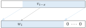 |
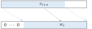 |
(a) Logical shift left: w = v << x. |
(b) Logical shift right: w = v >>> x. |
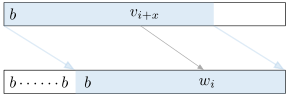 |
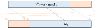 |
(c) Arithmetic shift right: w = v >> x. |
(d) Rotate right: w = v #>> x. |
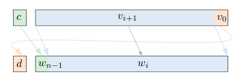 | |
(e) Rotate right extended by 1 place: (d,w) = word_rrx (c,v). | |
Arithmetic and orderings. The arithmetic operations are: addition, subtraction, unary minus (two's complement), logarithm (base-2), multiplication, modulus and division (signed and unsigned). These operations are defined with respect to the natural numbers. For example, word addition is defined by:
|- !v w. v + w = n2w (w2n v + w2n w)
The + on the left-hand side is word addition and on the right
it is natural number addition.
All of the standard word orderings are provided, with signed and
unsigned versions of $<$, $\leq$, $>$ and $\geq$. The unsigned
versions are suffixed with a plus; for example, <+ is unsigned
“less than”.
Constants. The word theory also defines a few word constants:
| Constant | Value | Binary |
|---|---|---|
word_T or UINT_MAXw | $2^l - 1$ | $11\cdots 11$ |
word_L or INT_MINw | $2^{l-1}$ | $10\cdots 00$ |
word_H or INT_MAXw | $2^{l-1} - 1$ | $01\cdots 11$ |
List of bit vector operations. A list of operations is provided in the table below.
| Operation | Symbol | Type | Description |
|---|---|---|---|
n2w | $\mathit{num}\to\worda$ | Map from a natural number | |
w2n | $\worda\to\mathit{num}$ | Map to a natural number | |
w2w | $\worda\to\wordb$ | Map word-to-word (unsigned) | |
sw2sw | $\worda\to\wordb$ | Map word-to-word (signed) | |
w2l | $\mathit{num}\to\worda\to\mathit{num}\,\mathit{list}$ | Map word to digit list | |
l2w | $\mathit{num}\to\mathit{num}\,\mathit{list}\to\worda$ | Map digit list to word | |
w2s | $\mathit{num}\to(\mathit{num}\to\mathit{char})\to\worda\to\mathit{string}$ | Map word to string | |
s2w | $\mathit{num}\to(\mathit{char}\to\mathit{num})\to\mathit{string}\to\worda$ | Map string to word | |
word_len | $\worda\to\mathit{num}$ | The word length | |
word_lsb | $\worda\to\mathit{bool}$ | The least significant bit | |
word_msb | $\worda\to\mathit{bool}$ | The most significant bit | |
word_bit | $\mathit{num}\to\worda\to\mathit{bool}$ | Test bit position | |
word_bits | -- | $\mathit{num}\to\mathit{num}\to\worda\to\worda$ | Select a bit field |
word_signed_bits | --- | $\mathit{num}\to\mathit{num}\to\worda\to\worda$ | Sign-extend selected bit field |
word_slice | '' | $\mathit{num}\to\mathit{num}\to\worda\to\worda$ | Set bits outside field to zero |
word_extract | >< | $\mathit{num}\to\mathit{num}\to\worda\to\wordb$ | Extract (cast) a bit field |
word_reverse | $\worda\to\worda$ | Reverse the bit order | |
bit_field_insert | $\mathit{num}\to\mathit{num}\to\worda\to\wordb\to\wordb$ | Insert a bit field | |
word_modify | $(\mathit{num}\to\mathit{bool}\to\mathit{bool})\to\worda\to\worda$ | Apply a function to each bit | |
word_join | $\worda\to\wordb\to\fcp{\mathit{bool}}{\alpha+\beta}$ | Join words | |
word_concat | @@ | $\worda\to\wordb\to\wordc$ | Concatenate words |
concat_word_list | $\worda\,\mathit{list}\to\wordb$ | Concatenate list of words | |
word_replicate | $\mathit{num}\to\worda\to\wordb$ | Replicate word | |
word_or | || | $\worda\to\worda\to\worda$ | Bitwise disjunction |
word_xor | ?? | $\worda\to\worda\to\worda$ | Bitwise exclusive-or |
word_and | && | $\worda\to\worda\to\worda$ | Bitwise conjunction |
word_nor | ~|| | $\worda\to\worda\to\worda$ | Bitwise NOR |
word_xnor | ~?? | $\worda\to\worda\to\worda$ | Bitwise XNOR |
word_nand | ~&& | $\worda\to\worda\to\worda$ | Bitwise NAND |
word_reduce | $(\mathit{bool}\to\mathit{bool}\to\mathit{bool})\to\worda\to\fcp{\mathit{bool}}{1}$ | Word reduction | |
reduce_or | $\worda\to\fcp{\mathit{bool}}{1}$ | Disjunction reduction | |
reduce_xor | $\worda\to\fcp{\mathit{bool}}{1}$ | Exclusive-or reduction | |
reduce_and | $\worda\to\fcp{\mathit{bool}}{1}$ | Conjunction reduction | |
reduce_nor | $\worda\to\fcp{\mathit{bool}}{1}$ | NOR reduction | |
reduce_xnor | $\worda\to\fcp{\mathit{bool}}{1}$ | XNOR reduction | |
reduce_nand | $\worda\to\fcp{\mathit{bool}}{1}$ | NAND reduction | |
word_1comp | ~ | $\worda\to\worda$ | One's complement |
word_2comp | - | $\worda\to\worda$ | Two's complement |
word_add | + | $\worda\to\worda\to\worda$ | Addition |
word_sub | - | $\worda\to\worda\to\worda$ | Subtraction |
word_mul | * | $\worda\to\worda\to\worda$ | Multiplication |
word_div | // | $\worda\to\worda\to\worda$ | Division (unsigned) |
word_sdiv | / | $\worda\to\worda\to\worda$ | Division (signed) |
word_mod | $\worda\to\worda\to\worda$ | Modulus | |
word_log2 | $\worda\to\worda$ | Logarithm base-2 | |
word_lsl | << | $\worda\to\mathit{num}\to\worda$ | Logical shift left |
word_lsr | >>> | $\worda\to\mathit{num}\to\worda$ | Logical shift right |
word_asr | >> | $\worda\to\mathit{num}\to\worda$ | Arithmetic shift right |
word_ror | #>> | $\worda\to\mathit{num}\to\worda$ | Rotate right |
word_rol | #<< | $\worda\to\mathit{num}\to\worda$ | Rotate left |
word_rrx | $\mathit{bool}\#\worda\to\mathit{bool}\#\worda$ | Rotate right extended by 1 place | |
word_lt | < | $\worda\to\worda\to\mathit{bool}$ | Signed “less than” |
word_le | <= | $\worda\to\worda\to\mathit{bool}$ | Signed “less than or equal” |
word_gt | > | $\worda\to\worda\to\mathit{bool}$ | Signed “greater than” |
word_ge | >= | $\worda\to\worda\to\mathit{bool}$ | Signed “greater than or equal” |
word_lo | <+ | $\worda\to\worda\to\mathit{bool}$ | Unsigned “less than” |
word_ls | <=+ | $\worda\to\worda\to\mathit{bool}$ | Unsigned “less than or equal” |
word_hi | >+ | $\worda\to\worda\to\mathit{bool}$ | Unsigned “greater than” |
word_hs | >=+ | $\worda\to\worda\to\mathit{bool}$ | Unsigned “greater than or equal” |
Sequences
HOL provides theories for various kinds of sequences: finite lists, lazy lists, paths, and finite strings.
Lists
HOL lists are inductively defined finite sequences where each
element in a list has the same type. The theory list introduces
the unary type operator $\alpha\;\konst{list}$ by a type definition
and a standard collection of list processing functions are
defined. The primitive constructors NIL and CONS
   NIL  : 'a list
   CONS : 'a -> 'a list -> 'a list
are used to build lists and have been defined from the representing
type for lists. The HOL parser
has been specially modified to parse the expression [] into
NIL, to parse the expression h::t into CONS h t, and to
parse the expression [$t_1$;$t_2$;…;$t_n$] into
CONS $t_1$(CONS$t_2$ $\cdots$(CONS$t_n$NIL)$\cdots$).
The HOL printer
reverses these transformations.
Based on the inductive characterization of the type, the following
fundamental theorems about lists are proved and stored in the
theory list.
list_Axiom
  ⊢ ∀f0 f1. ∃h. h [] = f0 ∧ ∀a0 a1. h (a0::a1) = f1 a0 a1 (h a1)
list_INDUCT
  ⊢ ∀P. P [] ∧ (∀t. P t ⇒ ∀h. P (h::t)) ⇒ ∀l. P l
list_CASES
  ⊢ ∀l. l = [] ∨ ∃h t. l = h::t
CONS_11
  ⊢ ∀a0 a1 a0' a1'. a0::a1 = a0'::a1' ⇔ a0 = a0' ∧ a1 = a1'
NOT_NIL_CONS
  ⊢ ∀a1 a0. [] ≠ a0::a1
NOT_CONS_NIL
  ⊢ ∀a1 a0. a0::a1 ≠ []
The theorem list_Axiom shown above is analogous to the primitive
recursion theorem
on the natural numbers discussed above in Section
5.3.1.3. It states the validity of primitive recursive
definitions on lists, and can be used to justify any such
definition. The ML function new_recursive_definition uses this
theorem to do automatic
proofs of the existence of primitive recursive functions on lists
and then make constant specifications to introduce constants that
denote such functions.
The induction theorem for lists, list_INDUCT, provides the main
proof tool used to reason about operations that manipulate lists.
The theorem list_CASES is used to perform case analysis on
whether a list is empty or not.
The theorem CONS_11 shows that CONS is injective; the theorems
NOT_NIL_CONS and NOT_CONS_NIL show that NIL and CONS are
distinct, i.e., cannot give rise to the same structure. Together,
these three theorems are used for equational reasoning about
lists.
The predicate NULL and the selectors
HD and TL are defined in the theory list by
NULL
  ⊢ NULL [] ∧ ∀h t. ¬NULL (h::t)
HD
  ⊢ ∀h t. HD (h::t) = h
TL_DEF
  ⊢ TL [] = [] ∧ ∀h t. TL (h::t) = t
The nil-clause for the TL constant is included to make the
function total, but does represent a case that often needs to be
excluded. For example:
LIST_NOT_NIL
  ⊢ ∀ls. ls ≠ [] ⇔ ls = HD ls::TL ls
The following functions on lists are also defined in the theory
list.
Case expressions. Compound HOL expressions that branch based on whether a term is an empty or non-empty list have the surface syntax (roughly borrowed from ML)
   case e1
    of [] => e2
     | (h::t) => e3
Such an expression is translated to
$\mathtt{list\_CASE}\;e_1\;e_2\;(\lambda h\;t.\;e_3)$ where the
constant list_CASE is defined as follows:
list_case_def
  ⊢ (∀v f. list_CASE [] v f = v) ∧
     ∀a0 a1 v f. list_CASE (a0::a1) v f = f a0 a1
List membership.
Membership in a list, written using the MEM syntax, is
characterised as follows:
MEM
  ⊢ (∀x. MEM x [] ⇔ F) ∧ ∀x h t. MEM x (h::t) ⇔ x = h ∨ MEM x t
Concatenation of lists.
Binary list concatenation (APPEND) may also be denoted by the
infix operator ++; thus the expression L1 ++ L2 is translated
into APPEND L1 L2. The concatenation of a list of lists into a
list is achieved by FLAT. The special case where a single
element is appended to the end of a list (the “opposite” of
CONS, which adds elements to the front of a list), is
implemented by SNOC.
APPEND
  ⊢ (∀l. [] ⧺ l = l) ∧ ∀l1 l2 h. h::l1 ⧺ l2 = h::(l1 ⧺ l2)
FLAT
  ⊢ FLAT [] = [] ∧ ∀h t. FLAT (h::t) = h ⧺ FLAT t
SNOC
  ⊢ (∀x. SNOC x [] = [x]) ∧
     ∀x x' l. SNOC x (x'::l) = x'::SNOC x l
Numbers and lists.
The length (LENGTH) and size (list_size) of a list are related
notions. The size of a list takes account of the size of each
element of the list (given by parameter $f:\alpha\to\konst{num}$),
while the length of the list ignores the size of each list
element. The alternate length definition (LEN) is
tail-recursive. Numbers can also be used to index into lists,
extracting the element at the specified position.
LENGTH
  ⊢ LENGTH [] = 0 ∧ ∀h t. LENGTH (h::t) = SUC (LENGTH t)
LEN_DEF
  ⊢ (∀n. LEN [] n = n) ∧ ∀h t n. LEN (h::t) n = LEN t (n + 1)
list_size_def
  ⊢ (∀f0. list_size f0 [] = 0) ∧
     ∀f0 a0 a1.
       list_size f0 (a0::a1) = 1 + (f0 a0 + list_size f0 a1)
EL
  ⊢ (∀l. l❲0❳ = HD l) ∧ ∀l n. l❲SUC n❳ = (TL l)❲n❳
Note that the extraction of the $n$th element (as described in
the theorem EL) of a list starts its indexing from 0. If the
length of the list $\ell$ is less than or equal to n, the
result of `ℓ❲n❳` is unspecified. The special syntax with
the brackets hides the underlying constant, which is EL of type
:num -> 'a list -> 'a. It is legal to use the constant
explicitly, writing EL n ℓ.
The GENLIST constant can be used to generate a list of a
particular size, where the value of each element is independently
determined by reference to a function that takes natural numbers
(the set $\{0\dots n-1\}$) to element values:
GENLIST
  ⊢ (∀f. GENLIST f 0 = []) ∧
     ∀f n. GENLIST f (SUC n) = SNOC (f n) (GENLIST f n)
EL_GENLIST
  ⊢ ∀f n x. x < n ⇒ (GENLIST f n)❲x❳ = f x
Working with SNOC, and thus the definition above, can
occasionally be awkward, so a characterisation of GENLIST's
SUC clause in terms of CONS can also be useful:
GENLIST_CONS
  ⊢ GENLIST f (SUC n) = f 0::GENLIST (f ∘ SUC) n
For more on the “indexed” treatment of lists, see Section 5.4.1.2 below.
Mapping functions over lists.
There are functions for mapping a function $f:\alpha\to\beta$ over
a single list (MAP), a “partial” function
$f:\alpha\to\beta\,\mathsf{option}$ over a list (mapPartial), or
a function $f:\alpha\to\beta\to\gamma$ over two lists (MAP2):
MAP
  ⊢ (∀f. MAP f [] = []) ∧ ∀f h t. MAP f (h::t) = f h::MAP f t
mapPartial_def
  ⊢ (∀f. mapPartial f [] = []) ∧
     ∀f x xs.
       mapPartial f (x::xs) =
       case f x of
         NONE => mapPartial f xs
       | SOME y => y::mapPartial f xs
MAP2_DEF
  ⊢ (∀t2 t1 h2 h1 f.
        MAP2 f (h1::t1) (h2::t2) = f h1 h2::MAP2 f t1 t2) ∧
     (∀y f. MAP2 f [] y = []) ∧ ∀v5 v4 f. MAP2 f (v4::v5) [] = []
If passed lists of unequal length, MAP2 returns a list of length
equal to that of the shorter list.
Predicates over lists.
Predicates can be applied to lists in a universal sense (the
predicate must hold of every element in the list) or an
existential sense (the predicate must hold of some element in the
list). This functionality is supported by EVERY and EXISTS,
respectively. The elimination of all elements in list not
satisfying a given predicate is performed by FILTER.
EVERY_DEF
  ⊢ (∀P. EVERY P [] ⇔ T) ∧
     ∀P h t. EVERY P (h::t) ⇔ P h ∧ EVERY P t
EXISTS_DEF
  ⊢ (∀P. EXISTS P [] ⇔ F) ∧
     ∀P h t. EXISTS P (h::t) ⇔ P h ∨ EXISTS P t
FILTER
  ⊢ (∀P. FILTER P [] = []) ∧
     ∀P h t.
       FILTER P (h::t) =
       if P h then h::FILTER P t else FILTER P t
ALL_DISTINCT
  ⊢ (ALL_DISTINCT [] ⇔ T) ∧
     ∀h t. ALL_DISTINCT (h::t) ⇔ ¬MEM h t ∧ ALL_DISTINCT t
The predicate ALL_DISTINCT holds on a list just in case no
element in the list is equal to any other. A list can have its
duplicates removed through the use of the nub constant:
nub_def
  ⊢ nub [] = [] ∧
     ∀x l. nub (x::l) = if MEM x l then nub l else x::nub l
Relations over lists.
A binary relation on elements can be “lifted” to a relation on
lists of such elements with the LIST_REL constant:
LIST_REL_def
  ⊢ (LIST_REL R [] [] ⇔ T) ∧ (LIST_REL R (a::as) [] ⇔ F) ∧
     (LIST_REL R [] (b::bs) ⇔ F) ∧
     (LIST_REL R (a::as) (b::bs) ⇔ R a b ∧ LIST_REL R as bs)
This can be viewed as an application of EVERY:
LIST_REL_EVERY_ZIP
  ⊢ ∀R l1 l2.
       LIST_REL R l1 l2 ⇔
       LENGTH l1 = LENGTH l2 ∧ EVERY (UNCURRY R) (ZIP (l1,l2))
Acknowledging this view, the system overloads the name EVERY2
to map to the same constant.
> “EVERY2 (λm n. EVEN (m + n)) [1;2;3] [3;4;5]”;
val it = “LIST_REL (λm n. EVEN (m + n)) [1; 2; 3] [3; 4; 5]”:
   term
Some theorems in listTheory have names that reflect this.
Equally, LIST_REL can be seen as a test that checks the
relation at all relevant indices:
LIST_REL_EL_EQN
  ⊢ ∀R l1 l2.
       LIST_REL R l1 l2 ⇔
       LENGTH l1 = LENGTH l2 ∧ ∀n. n < LENGTH l1 ⇒ R l1❲n❳ l2❲n❳
Finally, there is a natural induction principle for this constant (as per Section 7.7.1, the tactic ``Induct_on `LIST_REL``` applies it):
LIST_REL_strongind
  ⊢ ∀R LIST_REL'.
       LIST_REL' [] [] ∧
       (∀h1 h2 t1 t2.
          R h1 h2 ∧ LIST_REL R t1 t2 ∧ LIST_REL' t1 t2 ⇒
          LIST_REL' (h1::t1) (h2::t2)) ⇒
       ∀a0 a1. LIST_REL R a0 a1 ⇒ LIST_REL' a0 a1
Folding.
Applying a binary function $f:\alpha\to\beta\to\beta$ pairwise
through a list and accumulating the result is known as folding.
At times, it is necessary to do this operation from left-to-right
(FOLDL), and at others the right-to-left direction (FOLDR) is
required.
FOLDL
  ⊢ (∀f e. FOLDL f e [] = e) ∧
     ∀f e x l. FOLDL f e (x::l) = FOLDL f (f e x) l
FOLDR
  ⊢ (∀f e. FOLDR f e [] = e) ∧
     ∀f e x l. FOLDR f e (x::l) = f x (FOLDR f e l)
List reversal.
The reversal of a list (REVERSE) and its tail recursive
counterpart REV are defined in list.
   REVERSE_DEF
     |- (REVERSE [] = []) /\
        (!h t. REVERSE (h::t) = REVERSE t ++ [h])
   REV_DEF
     |- (!acc. REV [] acc = acc) /\
        (!h t acc. REV (h::t) acc = REV t (h::acc))
Conversion to sets.
Lists can be converted to sets with the LIST_TO_SET constant,
which is overloaded to the prettier name set. The definition is
made by primitive recursion in listTheory:
> listTheory.LIST_TO_SET;
val it = ⊢ set [] = ∅ ∧ set (h::t) = h INSERT set t: thm
Note that MEM is an overloaded form of syntax such that
MEM x l is actually a pretty-printing of the underlying term
x ∈ set l.
Further support for translating between different kinds of
collections may be found in the container theory.
Pairs and lists.
Two lists of equal length may be component-wise paired by the
ZIP operation. As with MAP2, the result of zipping lists of
unequal lengths is a list whose length is that of the shorter
argument. The inverse operation, UNZIP, translates a list of
pairs into a pair of lists.
ZIP_def
  ⊢ (∀l2. ZIP ([],l2) = []) ∧ (∀l1. ZIP (l1,[]) = []) ∧
     ∀x1 l1 x2 l2. ZIP (x1::l1,x2::l2) = (x1,x2)::ZIP (l1,l2)
UNZIP_THM
  ⊢ UNZIP [] = ([],[]) ∧
     UNZIP ((x,y)::t) = (let (L1,L2) = UNZIP t in (x::L1,y::L2))
Alternate access.
Lists are essentially treated in a stack-like manner. However,
at times it is convenient to access the last element (LAST) of
a non-empty list directly. The last element of a non-empty list
is dropped by FRONT.
LAST_DEF
  ⊢ ∀h t. LAST (h::t) = if t = [] then h else LAST t
FRONT_DEF
  ⊢ FRONT [] = [] ∧
     ∀h t. FRONT (h::t) = if t = [] then [] else h::FRONT t
APPEND_FRONT_LAST
  ⊢ ∀l. l ≠ [] ⇒ FRONT l ⧺ [LAST l] = l
Joining the front part and the last element of a non-empty list
yields the original list. Both LAST and FRONT are
unspecified on empty lists.
Prefix checking.
The relation capturing whether a list $\ell_1$ is a prefix of
$\ell_2$ (isPREFIX) can be defined by recursion. The infix
symbols <<= (ASCII) and $\preccurlyeq$ (U+227C) can also be
used as notation for this partial order.
isPREFIX_THM
  ⊢ ([] ≼ l ⇔ T) ∧ (h::t ≼ [] ⇔ F) ∧
     (h1::t1 ≼ h2::t2 ⇔ h1 = h2 ∧ t1 ≼ t2)
The above theorem states that: the empty list is a prefix of any other list (clause 1); that no non-empty list is a prefix of the empty list (clause 2); and that a non-empty list is a prefix of another non-empty list if the first elements of the lists are the same, and if the tail of the first is a prefix of the tail of the second.
For a complete list of available theorems in list, see the
REFERENCE manual. Further development of list theory can be found
in rich_list.
List permutations and sorting
The sorting theory defines a notion of two lists being
permutations of each other, then defines a general notion of
sorting, then shows that Quicksort is a sorting function. The
mergesort theory defines Merge sort and shows that it is a
stable sorting function.
List permutation.
Two lists are in permutation if they have exactly the same
members, and each member has the same number of occurrences in
both lists. One definition (PERM) that captures this
relationship is the following:
PERM_DEF
  ⊢ ∀L1 L2. PERM L1 L2 ⇔ ∀x. FILTER ($= x) L1 = FILTER ($= x) L2
PERM_IND
  ⊢ ∀P. P [] [] ∧ (∀x l1 l2. P l1 l2 ⇒ P (x::l1) (x::l2)) ∧
         (∀x y l1 l2. P l1 l2 ⇒ P (x::y::l1) (y::x::l2)) ∧
         (∀l1 l2 l3. P l1 l2 ∧ P l2 l3 ⇒ P l1 l3) ⇒
         ∀l1 l2. PERM l1 l2 ⇒ P l1 l2
A derived induction theorem (PERM_IND) is very useful in proofs
about permutations.
Sorting.
A list is $R$-sorted if $R$ holds pairwise through the list.
This notion (SORTED) is captured by a recursive definition.
Then a function of type
('a -> 'a -> bool) -> 'a list -> 'a list
is a sorting function (SORTS) with respect to $R$ if it
delivers a permutation of its input, and the result is
$R$-sorted.
SORTED_DEF
  ⊢ (∀R. SORTED R [] ⇔ T) ∧ (∀x R. SORTED R [x] ⇔ T) ∧
     ∀y x rst R. SORTED R (x::y::rst) ⇔ R x y ∧ SORTED R (y::rst)
SORTS_DEF
  ⊢ ∀f R. SORTS f R ⇔ ∀l. PERM l (f R l) ∧ SORTED R (f R l)
Quicksort is defined in the usual functional programming style, and it is indeed a sorting function, provided $R$ is a transitive and total relation.
QSORT_DEF
  ⊢ (∀ord. QSORT ord [] = []) ∧
     ∀t ord h.
       QSORT ord (h::t) =
       (let
          (l1,l2) = PARTITION (λy. ord y h) t
        in
          QSORT ord l1 ⧺ [h] ⧺ QSORT ord l2)
QSORT_SORTS
  ⊢ ∀R. transitive R ∧ total R ⇒ SORTS QSORT R
The notion of $R$ holding pairwise through a list can be
expressed using the predicate adjacent, where
$\mathtt{adjacent}\;\ell\;a\;b$ holds if values $a$ and $b$
appear together (in that order) in list $\ell$. Then, we have
SORTED_adjacent
  ⊢ SORTED R L ⇔ adjacent L ⊆ᵣ R
where the $\subseteq\subr$ relation is the notion of
relation-subset (see Section 5.5.3). There are a
number of other theorems in listTheory about adjacency,
including for example:
adjacent_REVERSE
  ⊢ ∀xs a b. adjacent (REVERSE xs) a b ⇔ adjacent xs b a
adjacent_MAP
  ⊢ ∀xs a b f.
       adjacent (MAP f xs) a b ⇔ ∃x y. adjacent xs x y ∧ a = f x ∧ b = f y
Indexed lists
As mentioned earlier, lists can be indexed with the constant
EL, viewing lists as partial functions from natural numbers
(starting at 0!) into the element type. The definition is given
by primitive recursion over the index argument, in theorem EL:
EL
  ⊢ (∀l. l❲0❳ = HD l) ∧ ∀l n. l❲SUC n❳ = (TL l)❲n❳
The term underlying the pretty presentation $\ell\lbrbrak n\rbrbrak$ is $\mathtt{EL}\;n\;\ell$; and both forms can be used when writing terms. If desired, the pretty-printing with the “array-subscript” notation can be turned off by the invocation
val _ = clear_overloads_on "fEL"
Note that because of the use of HD and TL, the value of
$\ell\lbrbrak n\rbrbrak$ is unspecified when
$n \geq \mathtt{LENGTH}\;\ell$. Subsequently, many theorems
involving EL have preconditions to preclude this possibility.
For example, these theorems describing the relationship between
EL, MAP and MEM:
EL_MAP
  ⊢ ∀n l. n < LENGTH l ⇒ ∀f. (MAP f l)❲n❳ = f l❲n❳
MEM_EL
  ⊢ ∀l x. MEM x l ⇔ ∃n. n < LENGTH l ∧ x = l❲n❳
It is occasionally useful to be able to update lists at
particular positions, viewing them as similar to programming
language arrays. The relevant constant is LUPDATE, where the
term $\mathtt{LUPDATE}\;e\;n\;\ell$ has the same value as list
$\ell$, except that the $n$-th element of the list is equal to
$e$.
The definition illustrates the pretty syntax for the above
($\ell\lbrbrak n\mapsto e\rbrbrak$), and is given in three
clauses:
LUPDATE_def
  ⊢ (∀e n. []❲n ↦ e❳ = []) ∧ (∀e x l. (x::l)❲0 ↦ e❳ = e::l) ∧
     ∀e n x l. (x::l)❲SUC n ↦ e❳ = x::l❲n ↦ e❳
The definition implies that attempting to update a list at an index beyond the end of the list returns the input list unchanged.
The basic characterisation of the link between EL and LUPDATE
is
EL_LUPDATE
  ⊢ ∀ys x i k. ys❲k ↦ x❳❲i❳ = if i = k ∧ k < LENGTH ys then x else ys❲i❳
The pretty syntax supports chained or nested LUPDATE
applications using a list-like notation:
> “LUPDATE v1 k1 (LUPDATE v2 k2 ℓ)”;
<<HOL message: inventing new type variable names: 'a>>
val it = “ℓ❲k1 ↦ v1; k2 ↦ v2❳”: term
The indexedLists theory.
The indexedLists theory defines a number of extra constants
that are “aware” of lists as indexed values. Some of these
constants are:
   delN      : num -> 'a list -> 'a list
   findi     : 'a -> 'a list -> num
   LIST_RELi : (num -> 'a -> 'b -> bool) -> 'a list -> 'b list -> bool
   MAPi      : (num -> 'a -> 'b) -> 'a list -> 'b list
The findi constant
is such that $\mathtt{findi}\;e\;\ell$ returns the first index of
element $e$ within list $\ell$, or a number equal to $\ell$'s
length, if $e$ is not present. The definition is by recursion
over the structure of the input list:
findi_def
  ⊢ (∀x. findi x [] = 0) ∧
     ∀x h t. findi x (h::t) = if x = h then 0 else 1 + findi x t
The delN constant
is used to remove the $n$-th element from a list. It is also
defined by recursion over the structure of the input list:
delN_def
  ⊢ (∀i. delN i [] = []) ∧
     ∀i h t. delN i (h::t) = if i = 0 then t else h::delN (i − 1) t
The higher-order MAPi function
exemplifies another set of constants within the indexedLists
theory: its function parameter, which works on elements of the
list argument is given access to the index of the list element as
well as its value. A simple example use might be to generate a
numbered version of a list, using the term
$\mathtt{MAPi}\;(\lambda i\;e.\;(i,e))$. If this term were
applied to the list [a;c;d] the resulting value would be
[(0,a);(1,c);(2,d)].
An example theorem about MAPi relates it to MEM:
MEM_MAPi
  ⊢ ∀x f l. MEM x (MAPi f l) ⇔ ∃n. n < LENGTH l ∧ x = f n l❲n❳
Possibly infinite sequences (llist)
The theory llist contains the definition of a type of possibly
infinite sequences. This type is similar to the “lazy lists” of
programming languages like Haskell, hence the name of the theory.
The llist theory has a number of constants that are analogous
to constants in the theory of finite lists. The llist versions
of these constants have the same names, but with a capital 'L'
prepended. Thus, some of the core constants in this theory are:
   LNIL  : 'a llist
   LCONS : 'a -> 'a llist -> 'a llist
   LHD   : 'a llist -> 'a option
   LTL   : 'a llist -> 'a llist option
The LHD and LTL constants return NONE when applied to the
empty sequence, LNIL. This use of an option type is another
way of modelling the essential partiality of these constants.
(In the theory of lists, the analogous HD and TL functions
simply have unspecified values when applied to empty lists.)
The type llist is not inductive, and there is no primitive
recursion theorem supporting the definition of functions that
have domains of type llist. Rather, llist is a coinductive
type, and has an axiom that justifies the definition of
(co-)recursive functions that map into the llist type:
   llist_Axiom
     ⊢ ∀f. ∃g.
          (∀x. LHD (g x) = OPTION_MAP SND (f x)) ∧
          ∀x. LTL (g x) = OPTION_MAP (g ∘ FST) (f x)
An equivalent form of the above is
llist_Axiom_1
  ⊢ ∀f. ∃g. ∀x. g x = case f x of NONE => [||] | SOME (a,b) => b:::g a
Other constants in the theory llist include LMAP, LFINITE,
LNTH, LTAKE, LDROP, and LFILTER. Their types are
   LMAP    : ('a -> 'b) -> 'a llist -> 'b llist
   LFINITE : 'a llist -> bool
   LNTH    : num -> 'a llist -> 'a option
   LTAKE   : num -> 'a llist -> 'a list option
   LDROP   : num -> 'a llist -> 'a llist option
   LFILTER : ('a -> bool) -> 'a llist -> 'a llist
They are characterised by the following theorems
LMAP
  ⊢ (∀f. LMAP f [||] = [||]) ∧ ∀f h t. LMAP f (h:::t) = f h:::LMAP f t
LFINITE_THM
  ⊢ (LFINITE [||] ⇔ T) ∧ ∀h t. LFINITE (h:::t) ⇔ LFINITE t
LNTH_THM
  ⊢ (∀n. LNTH n [||] = NONE) ∧ (∀h t. LNTH 0 (h:::t) = SOME h) ∧
     ∀n h t. LNTH (SUC n) (h:::t) = LNTH n t
LTAKE_THM
  ⊢ (∀l. LTAKE 0 l = SOME []) ∧ (∀n. LTAKE (SUC n) [||] = NONE) ∧
     ∀n h t. LTAKE (SUC n) (h:::t) = OPTION_MAP (CONS h) (LTAKE n t)
LDROP_THM
  ⊢ (∀ll. LDROP 0 ll = SOME ll) ∧ (∀n. LDROP (SUC n) [||] = NONE) ∧
     ∀n h t. LDROP (SUC n) (h:::t) = LDROP n t
LFILTER_THM
  ⊢ (∀P. LFILTER P [||] = [||]) ∧
     ∀P h t. LFILTER P (h:::t) = if P h then h:::LFILTER P t else LFILTER P t
Concatenation.
Two lazy lists may be concatenated by LAPPEND (written below
using its infix Unicode form ++$_l$). If the first lazy list
is infinite, elements of the second are inaccessible in the
result. A lazy list of lazy lists can be flattened to a lazy
list by LFLATTEN.
LAPPEND
  ⊢ (∀x. [||] ++ₗ x = x) ∧ ∀h t x. h:::t ++ₗ x = h:::(t ++ₗ x)
LFLATTEN_THM
  ⊢ LFLATTEN [||] = [||] ∧ (∀tl. LFLATTEN ([||]:::t) = LFLATTEN t) ∧
     ∀h t tl. LFLATTEN ((h:::t):::tl) = h:::LFLATTEN (t:::tl)
Lists and lazy lists.
Mapping back and forth from lists to lazy lists is accomplished
by fromList and toList:
fromList_def
  ⊢ fromList [] = [||] ∧ ∀h t. fromList (h::t) = h:::fromList t
toList_THM
  ⊢ toList [||] = SOME [] ∧
     ∀h t. toList (h:::t) = OPTION_MAP (CONS h) (toList t)
Note that toList ll = NONE when ll is infinite.
Proof principles.
Finally, there are two very important proof principles for
proving that two llist values are equal. The first states that
two sequences are equal if they return the same prefixes of
length $n$ for all possible values of $n$:
LTAKE_EQ
  ⊢ ∀ll1 ll2. ll1 = ll2 ⇔ ∀n. LTAKE n ll1 = LTAKE n ll2
This theorem is subsequently used to derive the bisimulation principle:
LLIST_BISIMULATION
  ⊢ ∀ll1 ll2.
       ll1 = ll2 ⇔
       ∃R. R ll1 ll2 ∧
           ∀ll3 ll4.
             R ll3 ll4 ⇒
             ll3 = [||] ∧ ll4 = [||] ∨
             LHD ll3 = LHD ll4 ∧ R (THE (LTL ll3)) (THE (LTL ll4))
The principle of bisimulation states that two llist values
$l_1$ and $l_2$ are equal if (and only if) it is possible to find
a relation $R$ such that
- $R$ relates the two values, i.e., $R\;l_1\;l_2$; and
- if $R$ holds of any two values $l_3$ and $l_4$, then either
- both $l_3$ and $l_4$ are empty; or
- the head elements of $l_3$ and $l_4$ are the same, and the tails of those two values are again related by $R$
Of course, a possible $R$ would be equality itself, but the strength of this theorem is that other, more convenient relations can also be used.
Labelled paths (path)
The theory path defines a binary type operator
$(\alpha,\beta)\,\mathtt{path}$, which stands for possibly
infinite paths of the following form
$$ \alpha_1 \stackrel{\beta_1}{\longrightarrow} \alpha_2 \stackrel{\beta_2}{\longrightarrow} \alpha_3 \stackrel{\beta_3}{\longrightarrow} \cdots \alpha_n \stackrel{\beta_n}{\longrightarrow} \alpha_{n+1} \stackrel{\beta_{n+1}}{\longrightarrow} \cdots $$
The path type is thus an appropriate model for reduction
sequences, where the $\alpha$ parameter corresponds to “states”,
and the $\beta$ parameter corresponds to the labels on the
arrows.
The model of $(\alpha,\beta)\,\mathtt{path}$ is $\alpha \times ((\alpha\times\beta)\,\mathtt{llist})$. The type of paths has two constructors:
   stopped_at : 'a -> ('a,'b) path
   pcons      : 'a -> 'b -> ('a,'b) path -> ('a,'b) path
The stopped_at constructor returns a path containing just one
state, and no transitions. (Thus, the reduction sequence has
“stopped at” this state.) The pcons constructor takes a
state, a label, and a path, and returns a path which is now
headed by the state argument, and which moves from that state
via the label argument to the path. Graphically,
$\mathtt{pcons}\;x\;l\;p$ is equal to
$$ x \stackrel{l}{\longrightarrow} \underbrace{p_1 \stackrel{l_1}{\longrightarrow} p_2 \stackrel{l_2}{\longrightarrow} \cdots\quad}_p $$
Other constants defined in theory path include
   finite  : ('a,'b) path -> bool
   first   : ('a,'b) path -> 'a
   labels  : ('a,'b) path -> 'b llist
   last    : ('a,'b) path -> 'a
   length  : ('a,'b) path -> num option
   okpath  : ('a -> 'b -> 'a -> bool) -> ('a,'b) path -> bool
   pconcat : ('a,'b) path -> 'b -> ('a,'b) path -> ('a,'b) path
   pmap    : ('a -> 'c) -> ('b -> 'd) -> ('a,'b)path -> ('c,'d)path
The first function returns the first element of a path. There
always is such an element, and the defining equations are
first_thm
  ⊢ (∀x. first (stopped_at x) = x) ∧ ∀x r p. first (pcons x r p) = x
On the other hand, the last function does not always have a
well-specified value, though it still has nice characterising
equations:
last_thm
  ⊢ (∀x. last (stopped_at x) = x) ∧ ∀x r p. last (pcons x r p) = last p
The theorem for finite has a similar feel, but has a definite
value (F, or false) on infinite paths, whereas the value of
last on such paths is unspecified:
finite_thm
  ⊢ (∀x. finite (stopped_at x) ⇔ T) ∧
     ∀x r p. finite (pcons x r p) ⇔ finite p
The function pconcat concatenates two paths, linking them with
a provided label. If the first path is infinite, then the result
is equal to that first path. The defining equation is
pconcat_thm
  ⊢ (∀x lab p2. pconcat (stopped_at x) lab p2 = pcons x lab p2) ∧
     ∀x r p lab p2.
       pconcat (pcons x r p) lab p2 = pcons x r (pconcat p lab p2)
These equations are true even when the first argument to
pconcat is an infinite path.
The okpath predicate tests whether or not a path is a valid
transition given a ternary transition relation. Its
characterising theorem is
okpath_thm
  ⊢ ∀R. (∀x. okpath R (stopped_at x)) ∧
         ∀x r p. okpath R (pcons x r p) ⇔ R x r (first p) ∧ okpath R p
There is also an induction principle that simplifies reasoning about finite $R$-paths:
finite_okpath_ind
  ⊢ ∀R. (∀x. P (stopped_at x)) ∧
         (∀x r p.
            okpath R p ∧ finite p ∧ R x r (first p) ∧ P p ⇒ P (pcons x r p)) ⇒
         ∀sigma. okpath R sigma ∧ finite sigma ⇒ P sigma
One can show that a set P of paths are all $R$-paths with the
co-induction principle:
okpath_co_ind
  ⊢ ∀P. (∀x r p. P (pcons x r p) ⇒ R x r (first p) ∧ P p) ⇒
         ∀p. P p ⇒ okpath R p
Character strings (string)
The theory string defines a type of characters and a type of
finite strings built from those characters, along with a useful
suite of definitions for operating on strings.
Characters.
The type char is represented by the numbers less than 256.
Two constants are defined: CHR : $\konst{num}\to\konst{char}$
and ORD : $\konst{char}\to\konst{num}$. The following
theorems hold:
  CHR_ORD  |- !a. CHR (ORD a) = a
  ORD_CHR  |- !r. r < 256 = (ORD (CHR r) = r)
Character literals can also be entered using ML syntax, with a hash character immediately followed by a string literal of length one. Thus:
> load "stringTheory";
val it = (): unit
> val t = ``f #"c" #"\n"``;
<<HOL message: inventing new type variable names: 'a>>
val t = “f #"c" #"\n"”: term

> dest_comb ``#"\t"``;
val it = (“CHR”, “9”): term * term
Strings.
The type string is an alias for the type char list. All
functions and predicates over lists are thus available for use
over strings. Some of these constants are overloaded so that
they are printed (and can be parsed) with names that are more
appropriate for the particular case of lists of characters.
For example, NIL and CONS over strings have alternative
names EMPTYSTRING and STRING respectively:
   EMPTYSTRING : string
   STRING      : char -> string -> string
The HOL parser maps the syntax "" to EMPTYSTRING, and the HOL
printer inverts this. The parser expands string literals of the
form "$c_1\,c_2\,\ldots\,c_n$" to the compound term
$$ \mathtt{STRING}\;c_1\;(\mathtt{STRING}\;c_2\,\ldots\, (\mathtt{STRING}\;c_{n-1}\;(\mathtt{STRING}\; c_n\;\mathtt{EMPTYSTRING}))\,\ldots\,) $$
Of course, one could also write
> ``[#"a"; #"b"]``;
val it = “"ab"”: term
String literals can be constructed using the various special
escape sequences that are used in ML. For example, \n for the
newline character, and a backslash followed by three decimal
digits for characters of the given number.
> val t = ``"foo bar\n\001"``;
val t = “"foo bar\n\^A"”: term
Note that if one wants to use the control-character syntax with the caret that the pretty-printer has chosen to use in printing the given string, and this occurs inside a quotation, then the caret will need to be doubled. (See Section 8.1.3.)
As with numerals, string literals can be injected into other
types, where it might make sense to have string literals appear
to inhabit types in addition to the core system's string type.
Such literals can be written with different delimiters to make it
clear that such an injection has occurred. For more on this
facility, see the REFERENCE manual's description of the
add_strliteral_form function.
There is also a destructor function DEST_STRING for strings
which returns an option type:
DEST_STRING_def
  ⊢ DEST_STRING "" = NONE ∧
     ∀c rst. DEST_STRING (STRING c rst) = SOME (c,rst)
Case expressions. Compound HOL expressions that branch based on whether a term is an empty or non-empty string can be written with the surface syntax
   case s
    of "" => e1
     | STRING c rst => e2
Such an expression is actually a case-expression over the underlying list, and so the underlying constant is that for lists.
Length and concatenation.
A standard function LENGTH can be written STRLEN when applied
to a string, and APPEND can be written as STRCAT. There are
also theorems characterising these constants in stringTheory,
though they are simply instantiations of results from
listTheory:
   STRLEN_THM
     |- (STRLEN "" = 0) /\
        (STRLEN (STRING c s) = 1 + STRLEN s)

   STRCAT_EQNS =
     |- (STRCAT "" s = s) /\
        (STRCAT s "" = s) /\
        (STRCAT (STRING c s1) s2 = STRING c (STRCAT s1 s2))
Strings into numbers, and vice versa.
It is natural to want to convert strings to and from (natural)
numbers. Constants supporting this for a variety of bases ($2$,
$8$, $10$, and $16$) are defined in the theory
ASCIInumbersTheory. There the constants are named according to
the scheme
$$ \mathtt{num\_}\{\mathtt{to},\mathtt{from}\}\mathtt{\_}\{\mathtt{bin},\mathtt{oct},\mathtt{dec},\mathtt{hex}\}\mathtt{\_string} $$
making for a total of eight constants. The two decimal constants
are also available under the (overloaded) names toString and
toNum. The natural theorem expressing these last two are
inverse is
toNum_toString
  ⊢ ∀n. toNum (toString n) = n
and there is also a theorem specifying how long the strings
produced by toString will be:
LENGTH_num_to_dec_string
  ⊢ STRLEN (toString n) = if n = 0 then 1 else LOG 10 n + 1
Collections
Several different notions of a collection of elements are available in HOL: sets, multisets, relations, and finite maps.
Sets (pred_set)
An extensive development of set theory is available in the
theory pred_set. Sets are represented by functions of the type
$\alpha\to\konst{bool}$, i.e., they are so-called characteristic
functions.
One can use the type abbreviation $\alpha\;\konst{set}$ instead
of $\alpha\to\konst{bool}$. Sets may be finite or infinite. All
of the elements in a set must have the same type.
Set membership is the basic notion that formalized set theory
is based on. In HOL, membership is represented by a the infix
constant IN, defined in theory bool for convenience.
IN_DEF
  ⊢ $IN = (λx f. f x)
The IN operator is merely a way of applying the characteristic
function to an item, as the following trivial consequence of the
definition shows:
SPECIFICATION
  ⊢ ∀P x. x ∈ P ⇔ P x
Two sets are equal if they have the same elements.
EXTENSION
  ⊢ ∀s t. s = t ⇔ ∀x. x ∈ s ⇔ x ∈ t
The negation of set-membership is not a separate constant, but is
available as a convenient overload (in both ASCII and Unicode
forms). Thus, instead of writing ~(e IN s), one can instead
write e NOTIN s or e ∉ s.
Empty and universal sets.
The empty set is the characteristic function that is constantly
false. The constant EMPTY denotes the empty set; it may be
written as {} and ∅ (U+2205). The universal set, UNIV, on
a type is the characteristic function that is always true for
elements of that type.
EMPTY_DEF
  ⊢ ∅ = (λx. F)
UNIV_DEF
  ⊢ 𝕌(:α) = (λx. T)
In addition to UNIV (perhaps with a type annotation :'a set),
one may also write univ(:'a) to represent the universal set
over type :'a. The Unicode syntax 𝕌(:'a) means the same.
The Unicode symbol for $\mathbb{U}$ is U+1D54C, and may not exist
in many fonts.
One of these forms will be used to print UNIV by default. The
user trace (see Section 10.2) "Univ pretty-printing"
can be set to zero to cancel this behaviour. Additionally, the
trace "Unicode Univ printing" can be used to stop the U+1D54C
syntax from being used, even if the Unicode trace is set.
The symbols univ and 𝕌 are high-priority prefixes (see
Section 8.1.2.6), and overloaded patterns
(see Section 8.1.2.3) mapping a value
of the itself type to the corresponding UNIV constant. One
effect is that one can write things like
FINITE univ(:'a)
without the need for parentheses around FINITE's argument.
Insertion, union, and intersection.
The insertion (INSERT, written infix) of an element into a set
is defined with a set comprehension. Set comprehension is
discussed in the next subsection. Set union (UNION, written
infix) and intersection (INTER, also infix) are given their
usual definitions by set comprehension.
INSERT_DEF
  ⊢ ∀x s. x INSERT s = {y | y = x ∨ y ∈ s}
UNION_DEF
  ⊢ ∀s t. s ∪ t = {x | x ∈ s ∨ x ∈ t}
INTER_DEF
  ⊢ ∀s t. s ∩ t = {x | x ∈ s ∧ x ∈ t}
UNION and INTER are binary operations. Indexed union and
intersection operations, i.e., $\bigcup_{i\in P}$ and
$\bigcap_{i\in P}$ are provided by the definitions of BIGUNION
and BIGINTER.
BIGUNION
  ⊢ ∀P. BIGUNION P = {x | ∃s. s ∈ P ∧ x ∈ s}
BIGINTER
  ⊢ ∀P. BIGINTER P = {x | ∀s. s ∈ P ⇒ x ∈ s}
Both BIGUNION and BIGINTER reduce a set of sets to a set and
thus have the type
$((\alpha\to\konst{bool})\to\konst{bool})\to(\alpha\to\konst{bool})$.
Subsets.
Set inclusion (SUBSET, infix), proper set inclusion (PSUBSET,
infix), and power set (POW) are defined as follows:
SUBSET_DEF
  ⊢ ∀s t. s ⊆ t ⇔ ∀x. x ∈ s ⇒ x ∈ t
PSUBSET_DEF
  ⊢ ∀s t. s ⊂ t ⇔ s ⊆ t ∧ s ≠ t
POW_DEF
  ⊢ ∀set. POW set = {s | s ⊆ set}
Set difference and complement.
The difference between two sets (DIFF, infix) is defined by a
set comprehension. Based on that, the deletion of a single
element (DELETE, infix) from a set is straightforward. Since
the universe of a type is always available via UNIV, the
complement (COMPL) of a set may be taken.
DIFF_DEF
  ⊢ ∀s t. s DIFF t = {x | x ∈ s ∧ x ∉ t}
DELETE_DEF
  ⊢ ∀s x. s DELETE x = s DIFF {x}
COMPL_DEF
  ⊢ ∀P. COMPL P = 𝕌(:α) DIFF P
Functions on sets.
The image of a function $f:\alpha\to\beta$ on a set (IMAGE) is
defined with a set comprehension.
IMAGE_DEF
  ⊢ ∀f s. IMAGE f s = {f x | x ∈ s}
Injections, surjections, and bijections between sets are defined as follows:
INJ_DEF
  ⊢ ∀f s t.
       INJ f s t ⇔
       (∀x. x ∈ s ⇒ f x ∈ t) ∧ ∀x y. x ∈ s ∧ y ∈ s ⇒ f x = f y ⇒ x = y
SURJ_DEF
  ⊢ ∀f s t.
       SURJ f s t ⇔
       (∀x. x ∈ s ⇒ f x ∈ t) ∧ ∀x. x ∈ t ⇒ ∃y. y ∈ s ∧ f y = x
BIJ_DEF
  ⊢ ∀f s t. BIJ f s t ⇔ INJ f s t ∧ SURJ f s t
Finite sets.
The finite sets (FINITE) are defined inductively as those built
from the empty set by a finite number of insertions.
FINITE_DEF
  ⊢ ∀s. FINITE s ⇔ ∀P. P ∅ ∧ (∀s. P s ⇒ ∀e. P (e INSERT s)) ⇒ P s
A set is infinite iff it is not finite, and there is an
abbreviation in the system that parses "INFINITE s" into
"~FINITE s". The pretty-printer reverses this transformation.
The finite sets have an induction theorem:
FINITE_INDUCT
  ⊢ ∀P. P ∅ ∧ (∀s. FINITE s ∧ P s ⇒ ∀e. e ∉ s ⇒ P (e INSERT s)) ⇒
         ∀s. FINITE s ⇒ P s
As mentioned, set operations apply to both finite and infinite
sets. However, some operations, such as cardinality (CARD),
are only defined for finite sets. (See Section
6.1.2 for the theory of cardinality of possibly
infinite sets.)
CARD_DEF
  ⊢ CARD ∅ = 0 ∧
     ∀s. FINITE s ⇒
         ∀x. CARD (x INSERT s) = if x ∈ s then CARD s else SUC (CARD s)
Since the finite and infinite sets are dealt with uniformly in
pred_set, properties of operations on finite sets must
explicitly include constraints about finiteness. For example
the following theorem relating cardinality and subsets is only
true for finite sets.
CARD_PSUBSET
  ⊢ ∀s. FINITE s ⇒ ∀t. t ⊂ s ⇒ CARD t < CARD s
An extensive suite of theorems dealing with finiteness and
cardinality is available in pred_set.
Cross product.
The product of two sets (CROSS, infix) is defined with a set
comprehension.
CROSS_DEF
  ⊢ ∀P Q. P × Q = {p | FST p ∈ P ∧ SND p ∈ Q}
Cardinality and cross product are related by the following theorem:
CARD_CROSS
  ⊢ ∀P Q. FINITE P ∧ FINITE Q ⇒ CARD (P × Q) = CARD P * CARD Q
Recursive functions on sets.
Recursive functions on sets may be defined by wellfounded
recursion. Usually, the totality of such a function is
established by measuring the cardinality of the (finite) set.
However, another theorem may be used to justify a fold (ITSET)
for finite sets. Provided a function $f:\alpha\to\beta\to\beta$
obeys a condition known as left-commutativity, namely,
$f\;x\;(f\;y\;z) = f\;y\;(f\;x\;z)$, then $f$ can be applied by
folding it on the set in a tail-recursive fashion.
ITSET_THM
  ⊢ ∀s f b.
       FINITE s ⇒
       ITSET f s b = if s = ∅ then b else ITSET f (REST s) (f (CHOICE s) b)

ITSET_EMPTY
  ⊢ ∀f b. ITSET f ∅ b = b

COMMUTING_ITSET_INSERT
  ⊢ ∀f s.
       (∀x y z. f x (f y z) = f y (f x z)) ∧ FINITE s ⇒
       ∀x b. ITSET f (x INSERT s) b = ITSET f (s DELETE x) (f x b)
A recursive version is also available:
COMMUTING_ITSET_RECURSES
  ⊢ ∀f e s b.
       (∀x y z. f x (f y z) = f y (f x z)) ∧ FINITE s ⇒
       ITSET f (e INSERT s) b = f e (ITSET f (s DELETE e) b)
For the full derivation, see the sources of pred_set. The
definition of ITSET allows, for example, the definition of
summing the results of a function on a finite set of elements,
from which a recursive characterization and other useful
theorems are derived.
SUM_IMAGE_DEF
  ⊢ ∀f s. ∑ f s = ITSET (λe acc. f e + acc) s 0
SUM_IMAGE_THM
  ⊢ ∀f. ∑ f ∅ = 0 ∧
         ∀e s. FINITE s ⇒ ∑ f (e INSERT s) = f e + ∑ f (s DELETE e)
Other definitions and theorems.
There are more definitions in pred_set, but they are not as
heavily used as the ones presented here. Similarly, most
theorems in pred_set relate the various common set operations
to each other, but do not express any deep theorems of set
theory.
However, one notable theorem is Koenig's Lemma, which states
that every finitely branching infinite tree has an infinite
path. There are many ways to formulate this theorem, depending
on how the notion of tree is formalized. In HOL's formulation,
the tree is characterised by making various assumptions about
the finite-ness or otherwise of elements reachable using a
relation R. Then the following version of Koenig's Lemma is
stated and proved:
KoenigsLemma
  ⊢ ∀R. (∀x. FINITE {y | R x y}) ⇒
         ∀x. INFINITE {y | R꙳ x y} ⇒ ∃f. f 0 = x ∧ ∀n. R (f n) (f (SUC n))
Syntax for sets
The special purpose set-theoretic notations
{$t_1; t_2; \ldots; t_n$} and {$t$|$p$} are
recognized by the HOL parser and printer when the theory
pred_set is loaded.
The normal interpretation of {$t_1;t_2;\ldots;t_n$} is the
finite set containing just $t_1, t_2, \ldots, t_n$. This can be
modelled by starting with the empty set and performing a
sequence of insertions. For example, {1;2;3;4} parses to
1 INSERT (2 INSERT (3 INSERT (4 INSERT EMPTY)))
Set comprehensions.
The normal interpretation of {$t$|$p$} is the set of all
$t$s such that $p$. In HOL, such syntax parses to:
GSPEC(\($x_1$,…,$x_n$).($t$,$p$))
where $x_1, \ldots, x_n$ are those free variables that occur in both $t$ and $p$ if both have at least one free variable. If $t$ or $p$ has no free variables, then $x_1,\ldots,x_n$ are taken to be the free variables of the other term. If both terms have free variables, but there is no overlap, then an error results. The order in which the variables are listed in the variable structure of the paired abstraction is an unspecified function of the structure of $t$ (it is approximately left to right). For example,
{p+q | p < q /\ q < r}
parses to:
GSPEC(\(p,q). ((p+q), (p < q /\ q < r)))
where GSPEC is characterized by:
GSPECIFICATION
  ⊢ ∀f v. v ∈ GSPEC f ⇔ ∃x. (v,T) = f x
This somewhat cryptic specification can be understood by exercising an example. The syntax
a IN {p+q | p < q /\ q < r}
is mapped by the HOL parser to
a IN GSPEC(\(p,q). ((p+q), (p < q /\ q < r)))
which, by GSPECIFICATION, is equal to
?x. (a,T) = (\(p,q). ((p+q), (p < q /\ q < r))) x
The existentially quantified variable x has a pair type, so it
can be replaced by a pair (p,q) and a paired-$\beta$-reduction
can be performed, yielding
?(p,q). (a,T) = ((p+q), (p < q /\ q < r))
which is equal to the intended meaning of the original syntax:
?(p,q). (a = p+q) /\ (p < q /\ q < r)
Unambiguous set comprehensions.
There is also an unambiguous set comprehension syntax, which
allows the user to specify which variables are to be quantified
over in the abstraction that is the argument of GSPEC. Terms
of the form
{ t | vs | P }
generate sets containing values of the form given by t, where
the variables mentioned in vs must satisfy the constraint
P. For example, the set
{ x + y | x | x < y }
is the set of numbers from y up to but not including 2 * y.
The set can be “read” computationally: draw out all those x
that are less than y, and to each such x add y, thereby
generating a set of numbers.
In the example above, the underlying GSPEC term will be
GSPEC (\x. (x + y, x < y))
The vs component of the unambiguous notation must be a single
“variable structure” that might appear underneath a possibly
paired abstraction as in Section 5.2.3.1. In other
words, this
{ x + y | (x,y) | x < y }
is fine, but this
{ x + y | x y | x < y }
will raise an error. (Additionally, the outermost parentheses
around pairs in the vs position can be omitted.)
The unambiguous notation is printed by the pretty-printer
whenever the set to be printed can not be expressed with the
default notation, or if the trace variable with name
pp_unambiguous_comprehensions is set to 1. (If the same
trace is set to 2, then the unambiguous notation will never be
used.)
Decision procedure for set-theoretic theorems
HOL provides some tools (in bossLib) to automate the proof of
some routine pred_set theorems by a reduction to first-order
logic, ported from HOL Light. They are based on metisLib (see
Section 8.4.2). Below are the entry-points: (see
the REFERENCE manual for more details.)
   SET_TAC     : thm list -> tactic
   ASM_SET_TAC : thm list -> tactic
   SET_RULE    : term -> thm
The difference between SET_TAC and ASM_SET_TAC is that the
latter one also makes use of assumptions. With them, many
simple set-theoretic results can be directly proved without
finding needed lemmas in pred_setTheory. For instance, a
simple lemma from util_probTheory:
Theorem DISJOINT_RESTRICT_L :
  !s t c. DISJOINT s t ==> DISJOINT (s INTER c) (t INTER c)
Proof SET_TAC []
QED
Multisets (bag)
Multisets, also known as bags, are similar to sets, except that they allow repeat occurrences of an element. Whereas sets are represented by functions of type $\alpha\to\konst{bool}$, which signal the presence, or absence, of an element, multisets are represented by functions of type $\alpha\to\konst{num}$, which give the multiplicity of each element in the multiset. Multisets may be finite or infinite.
The type abbreviations $\alpha\;\konst{multiset}$ and $\alpha\;\konst{bag}$ can be used instead of $\alpha\to\konst{num}$.
Empty multiset. The empty bag has no elements. Thus, the function implementing it returns $0$ for every input.
EMPTY_BAG
  ⊢ {||} = K 0
The special syntax {||} (the analogue of [] for lists, and
{} for sets) is used for both printing and parsing, but the
underlying constant is indeed called EMPTY_BAG, and this name
can also be passed to the parser.
Membership.
Much of the theory can be based on the notion of membership in a
bag. There are two notions: does an element occur at least $n$
times in a bag (BAG_INN); and does an element occur in a bag
at all (BAG_IN).
BAG_INN
  ⊢ ∀e n b. BAG_INN e n b ⇔ b e ≥ n
BAG_IN
  ⊢ ∀e b. e ⋲ b ⇔ BAG_INN e 1 b
Two bags are equal if all elements have the same tally.
BAG_EXTENSION
  ⊢ ∀b1 b2. b1 = b2 ⇔ ∀n e. BAG_INN e n b1 ⇔ BAG_INN e n b2
Sub-multiset.
A sub-bag relationship (SUB_BAG) holds between $b_1$ and $b_2$
provided that every element in $b_1$ occurs at least as often in
$b_2$. The notion of a proper sub-bag (PSUB_BAG) is easily
defined.
SUB_BAG
  ⊢ ∀b1 b2. b1 ≤ b2 ⇔ ∀x n. BAG_INN x n b1 ⇒ BAG_INN x n b2
PSUB_BAG
  ⊢ ∀b1 b2. b1 < b2 ⇔ b1 ≤ b2 ∧ b1 ≠ b2
Insertion.
Inserting an element into a bag (BAG_INSERT) updates the tally
for that element and leaves the others unchanged.
BAG_INSERT
  ⊢ ∀e b. BAG_INSERT e b = (λx. if x = e then b e + 1 else b x)
Explicitly-given multisets are supported by the syntax
{|$t_1; t_2; \ldots; t_n$|}, where there may, of course, be
repetitions. This is modelled by starting with the empty
multiset and performing a sequence of insertions. For example,
{|1; 2; 3; 2; 1|} parses to
   BAG_INSERT 1 (BAG_INSERT 2 (BAG_INSERT 3
                                 (BAG_INSERT 2 (BAG_INSERT 1 {||}))))
Union and difference.
The union (BAG_UNION) and difference (BAG_DIFF) operations
on bags both reduce to an arithmetic calculation on their
elements. Deleting a single element from a bag may be expressed
by taking the multiset difference with a single-element
multiset; however, there is also a relational presentation
(BAG_DELETE) which relates its first and last arguments only
if the first contains exactly one more occurrence of the middle
argument than the last. This is not the same as using
BAG_DIFF to remove a one-element bag because it insists that
the element being removed actually appear in the larger bag.
BAG_UNION
  ⊢ ∀b c. b ⊎ c = (λx. b x + c x)
BAG_DIFF
  ⊢ ∀b1 b2. b1 − b2 = (λx. b1 x − b2 x)
BAG_DELETE
  ⊢ ∀b0 e b. BAG_DELETE b0 e b ⇔ b0 = BAG_INSERT e b
Intersection, merge, and filter.
The intersection of two bags (BAG_INTER) takes the pointwise
minimum. The dual operation, merging (BAG_MERGE), takes the
pointwise maximum. A bag can be ‘filtered’ by a set to return
the bag where all the elements not in the set have been dropped
(BAG_FILTER).
BAG_INTER
  ⊢ ∀b1 b2. BAG_INTER b1 b2 = (λx. if b1 x < b2 x then b1 x else b2 x)
BAG_MERGE
  ⊢ ∀b1 b2. BAG_MERGE b1 b2 = (λx. if b1 x < b2 x then b2 x else b1 x)
BAG_FILTER_DEF
  ⊢ ∀P b. BAG_FILTER P b = (λe. if P e then b e else 0)
Sets and multisets. Moving between bags and sets is accomplished by the following two definitions.
SET_OF_BAG
  ⊢ ∀b. SET_OF_BAG b = (λx. x ⋲ b)
BAG_OF_SET
  ⊢ ∀P. BAG_OF_SET P = (λx. if x ∈ P then 1 else 0)
Image. Taking the image of a function on a multiset to get a new multiset seems to be simply a matter of applying the function to each element of the multiset. However, there is a problem if $f$ is non-injective and the multiset is infinite. For example, take the multiset consisting of all the natural numbers and apply $\lambda x.\;1$ to each element. The resulting multiset would hold an infinite number of $1$s. To avoid this requires some constraints: for example, stipulating that the function be only finitely non-injective, or that the input multiset be finite. Such conditions would be onerous in proof; the compromise is to map the multipicity of problematic elements to $0$.
BAG_IMAGE_DEF
  ⊢ ∀f b.
       BAG_IMAGE f b =
       (λe.
          (let
             sb = BAG_FILTER (λe0. f e0 = e) b
           in
             if FINITE_BAG sb then BAG_CARD sb else 1))
Finite multisets.
The finite multisets (FINITE_BAG) are defined inductively as
those built from the empty bag by a finite number of insertions.
FINITE_BAG
  ⊢ ∀b. FINITE_BAG b ⇔ ∀P. P {||} ∧ (∀b. P b ⇒ ∀e. P (BAG_INSERT e b)) ⇒ P b
The finite multisets have an induction theorem, and also a strong induction theorem.
FINITE_BAG_INDUCT
  ⊢ ∀P. P {||} ∧ (∀b. P b ⇒ ∀e. P (BAG_INSERT e b)) ⇒ ∀b. FINITE_BAG b ⇒ P b

STRONG_FINITE_BAG_INDUCT
  ⊢ ∀P. P {||} ∧ (∀b. FINITE_BAG b ∧ P b ⇒ ∀e. P (BAG_INSERT e b)) ⇒
         ∀b. FINITE_BAG b ⇒ P b
The cardinality (BAG_CARD) of a multiset counts the total
number of occurrences. It is only specified for finite
multisets.
BAG_CARD_THM
  ⊢ BAG_CARD {||} = 0 ∧
     ∀b. FINITE_BAG b ⇒ ∀e. BAG_CARD (BAG_INSERT e b) = BAG_CARD b + 1
Recursive functions on multisets.
Recursive functions on multiset may be defined by wellfounded
recursion. Usually, the totality of such a function is
established by measuring the cardinality of the (finite)
multiset. However, a fold (ITBAG) for finite sets is provided.
Provided a function $f:\alpha\to\beta\to\beta$ obeys a condition
known as left-commutativity, namely,
$f\;x\;(f\;y\;z) = f\;y\;(f\;x\;z)$, then $f$ can be applied by
folding it on the multiset in a tail-recursive fashion.
ITBAG_EMPTY
  ⊢ ∀f acc. ITBAG f {||} acc = acc
COMMUTING_ITBAG_INSERT
  ⊢ ∀f b.
       (∀x y z. f x (f y z) = f y (f x z)) ∧ FINITE_BAG b ⇒
       ∀x a. ITBAG f (BAG_INSERT x b) a = ITBAG f b (f x a)
A recursive version is also available:
COMMUTING_ITBAG_RECURSES
  ⊢ ∀f e b a.
       (∀x y z. f x (f y z) = f y (f x z)) ∧ FINITE_BAG b ⇒
       ITBAG f (BAG_INSERT e b) a = f e (ITBAG f b a)
Relations (relation)
Mathematical relations can be represented in HOL by the type
$\alpha\to\beta\to\konst{bool}$. (In most applications, the
type of a relation is an instance of
$\alpha\to\alpha\to\konst{bool}$, but the extra generality
doesn't hurt.) The theory relation provides definitions of
basic properties and operations on relations, defines various
kinds of orders and closures, defines basic properties of relation transformers,
defines wellfoundedness and proves the wellfounded recursion theorem, and
develops some basic results used in Term Rewriting.
Basic properties. The following basic properties of relations are defined.
transitive_def
  ⊢ ∀R. transitive R ⇔ ∀x y z. R x y ∧ R y z ⇒ R x z
reflexive_def
  ⊢ ∀R. reflexive R ⇔ ∀x. R x x
irreflexive_def
  ⊢ ∀R. irreflexive R ⇔ ∀x. ¬R x x
symmetric_def
  ⊢ ∀R. symmetric R ⇔ ∀x y. R x y ⇔ R y x
antisymmetric_def
  ⊢ ∀R. antisymmetric R ⇔ ∀x y. R x y ∧ R y x ⇒ x = y
equivalence_def
  ⊢ ∀R. equivalence R ⇔ reflexive R ∧ symmetric R ∧ transitive R
trichotomous
  ⊢ ∀R. trichotomous R ⇔ ∀a b. R a b ∨ R b a ∨ a = b
total_def
  ⊢ ∀R. total R ⇔ ∀x y. R x y ∨ R y x
Basic operations.
The following basic operations on relations are defined: the
empty relation (EMPTY_REL, or $\emptyset\subr$), relation
composition (O, or $\circ\subr$, infix), inversion (inv, or
$\_^{\mathsf{T}}$ (suffix superscript ‘T’)), domain (RDOM),
and range (RRANGE).
EMPTY_REL_DEF
  ⊢ ∀x y. ∅ᵣ x y ⇔ F
O_DEF
  ⊢ ∀R1 R2 x z. (R1 ∘ᵣ R2) x z ⇔ ∃y. R2 x y ∧ R1 y z
inv_DEF
  ⊢ ∀R x y. Rᵀ x y ⇔ R y x
RDOM_DEF
  ⊢ ∀R x. RDOM R x ⇔ ∃y. R x y
RRANGE
  ⊢ ∀R y. RRANGE R y ⇔ ∃x. R x y
Set operations lifted to work on relations include subset
(RSUBSET, or $\subseteq\subr$, infix), union (RUNION, or
$\cup\subr$, infix), intersection (RINTER, or $\cap\subr$,
infix), complement (RCOMPL), and universe (RUNIV, or
$\mathbb{U}\subr$).
RSUBSET
  ⊢ ∀R1 R2. R1 ⊆ᵣ R2 ⇔ ∀x y. R1 x y ⇒ R2 x y
RUNION
  ⊢ ∀R1 R2 x y. (R1 ∪ᵣ R2) x y ⇔ R1 x y ∨ R2 x y
RINTER
  ⊢ ∀R1 R2 x y. (R1 ∩ᵣ R2) x y ⇔ R1 x y ∧ R2 x y
RCOMPL
  ⊢ ∀R x y. RCOMPL R x y ⇔ ¬R x y
RUNIV
  ⊢ ∀x y. 𝕌ᵣ x y ⇔ T
Orders.
A sequence of definitions capturing various notions of order are
made in relation.
PreOrder
  ⊢ ∀R. PreOrder R ⇔ reflexive R ∧ transitive R
Order
  ⊢ ∀Z. Order Z ⇔ antisymmetric Z ∧ transitive Z
WeakOrder
  ⊢ ∀Z. WeakOrder Z ⇔ reflexive Z ∧ antisymmetric Z ∧ transitive Z
StrongOrder
  ⊢ ∀Z. StrongOrder Z ⇔ irreflexive Z ∧ transitive Z
LinearOrder
  ⊢ ∀R. LinearOrder R ⇔ Order R ∧ trichotomous R
WeakLinearOrder
  ⊢ ∀R. WeakLinearOrder R ⇔ WeakOrder R ∧ trichotomous R
StrongLinearOrder
  ⊢ ∀R. StrongLinearOrder R ⇔ StrongOrder R ∧ trichotomous R
Closures.
The transitive closure (TC) of a relation
$R:\alpha\to\alpha\to\konst{bool}$ is defined inductively, as
the least relation including $R$ and closed under transitivity.
Similarly, the reflexive-transitive closure (RTC) is defined
to be the least relation closed under transitivity and
reflexivity. The ASCII syntax for the transitive closure
R^+ is meant to suggest the prettier R⁺. Similarly, R^*
is meant to suggest R∗. Indeed, with Unicode enabled,
transitive closure will print with a superscript +, and RTC
will print as a superscript asterisk.
From the underlying definitions, one can recover the initial rules:
TC_RULES
  ⊢ ∀R. (∀x y. R x y ⇒ R⁺ x y) ∧ ∀x y z. R⁺ x y ∧ R⁺ y z ⇒ R⁺ x z
RTC_RULES
  ⊢ ∀R. (∀x. R꙳ x x) ∧ ∀x y z. R x y ∧ R꙳ y z ⇒ R꙳ x z
RTC_RULES_RIGHT1
  ⊢ ∀R. (∀x. R꙳ x x) ∧ ∀x y z. R꙳ x y ∧ R y z ⇒ R꙳ x z
Notice that RTC_RULES, in keeping with the definition of
RTC, extends an R-step from x to y with a sequence of
R-steps from y to z to construct R* x z. The theorem
RTC_RULES_RIGHT1 first makes a sequence of R steps and then
a single R step to form R* x z. Similar alternative
theorems are proved for case analysis and induction.
For example, TC_CASES1 and TC_CASES2 in the following
decompose R+ x z to either R x y followed by R+ y z
(TC_CASES1) or R+ x y followed by R y z (TC_CASES2).
TC_CASES1
  ⊢ R⁺ x z ⇔ R x z ∨ ∃y. R x y ∧ R⁺ y z
TC_CASES2
  ⊢ R⁺ x z ⇔ R x z ∨ ∃y. R⁺ x y ∧ R y z

RTC_CASES1
  ⊢ ∀R x y. R꙳ x y ⇔ x = y ∨ ∃u. R x u ∧ R꙳ u y
RTC_CASES2
  ⊢ ∀R x y. R꙳ x y ⇔ x = y ∨ ∃u. R꙳ x u ∧ R u y
RTC_CASES_RTC_TWICE
  ⊢ ∀R x y. R꙳ x y ⇔ ∃u. R꙳ x u ∧ R꙳ u y
As well as the basic induction theorems for TC and RTC,
there are so-called strong induction theorems, which have
stronger induction hypotheses.
TC_INDUCT
  ⊢ ∀R P.
       (∀x y. R x y ⇒ P x y) ∧ (∀x y z. P x y ∧ P y z ⇒ P x z) ⇒
       ∀u v. R⁺ u v ⇒ P u v
RTC_INDUCT
  ⊢ ∀R P.
       (∀x. P x x) ∧ (∀x y z. R x y ∧ P y z ⇒ P x z) ⇒
       ∀x y. R꙳ x y ⇒ P x y
TC_STRONG_INDUCT
  ⊢ ∀R P.
       (∀x y. R x y ⇒ P x y) ∧
       (∀x y z. P x y ∧ P y z ∧ R⁺ x y ∧ R⁺ y z ⇒ P x z) ⇒
       ∀u v. R⁺ u v ⇒ P u v
RTC_STRONG_INDUCT
  ⊢ ∀R P.
       (∀x. P x x) ∧ (∀x y z. R x y ∧ R꙳ y z ∧ P y z ⇒ P x z) ⇒
       ∀x y. R꙳ x y ⇒ P x y
Variants of these induction theorems are also available which break apart the closure from the left or right, as for the case analysis theorems.
The reflexive (RC) and symmetric closures (SC) are
straightforward to define. The equivalence closure (EQC) is
the symmetric then transitive then reflexive closure of $R$.
When applied to an argument, as in EQC R, EQC is written
with the suffix ^=. Note how the suffix binds more tightly
than function application, so that in EQC_DEF, RC really is
applied to the transitive closure of the symmetric closure of
R.
RC_DEF
  ⊢ ∀R x y. RC R x y ⇔ x = y ∨ R x y
SC_DEF
  ⊢ ∀R x y. SC R x y ⇔ R x y ∨ R y x
EQC_DEF
  ⊢ ∀R. R^= = RC (SC R)⁺
These closures are an example of a relation transformer, which are of type
$b:(\alpha\to\alpha\to\konst{bool})\to\alpha\to\alpha\to\konst{bool}$. A
transformer is monotone (rmonotone) if it respects RSUBSET. A transformer
preserves a property P (rpreserves) if relations with property P continue
to have property P after being transformed. Finally, a transformer b is the
closure of a property P when it maps all relations R to their P-closures.
Theorems for these transformer properties involving the relation properties/closures
above have been added to the simpset.
rmonotone_def
  ⊢ ∀b. rmonotone b ⇔ ∀R1 R2. R1 ⊆ᵣ R2 ⇒ b R1 ⊆ᵣ b R2
rpreserves_def
  ⊢ ∀P b. rpreserves P b ⇔ ∀R. P R ⇒ P (b R)
is_closure_op_def
  ⊢ ∀P C.
       is_closure_op P C ⇔
       (∀R. P (C R)) ∧ (∀R. R ⊆ᵣ C R) ∧ ∀R1 R2. P R2 ∧ R1 ⊆ᵣ R2 ⇒ C R1 ⊆ᵣ R2
Wellfounded relations.
A relation $R$ is wellfounded (WF) if every non-empty set has
an $R$-minimal element. Wellfoundedness is used to justify the
principle of wellfounded induction (WF_INDUCTION_THM).
WF_DEF
  ⊢ ∀R. WF R ⇔ ∀B. (∃w. B w) ⇒ ∃min. B min ∧ ∀b. R b min ⇒ ¬B b
WF_INDUCTION_THM
  ⊢ ∀R. WF R ⇒ ∀P. (∀x. (∀y. R y x ⇒ P y) ⇒ P x) ⇒ ∀x. P x
The wellfounded part (WFP) of a relation can be inductively
defined, from which its rules, case-analysis theorem and
induction theorems may be derived.
WFP_DEF
  ⊢ ∀R a. WFP R a ⇔ ∀P. (∀x. (∀y. R y x ⇒ P y) ⇒ P x) ⇒ P a
WFP_RULES
  ⊢ ∀R x. (∀y. R y x ⇒ WFP R y) ⇒ WFP R x
WFP_CASES
  ⊢ ∀R x. WFP R x ⇔ ∀y. R y x ⇒ WFP R y
WFP_INDUCT
  ⊢ ∀R P. (∀x. (∀y. R y x ⇒ P y) ⇒ P x) ⇒ ∀x. WFP R x ⇒ P x
WFP_STRONG_INDUCT
  ⊢ ∀R. (∀x. WFP R x ∧ (∀y. R y x ⇒ P y) ⇒ P x) ⇒ ∀x. WFP R x ⇒ P x
Wellfoundedness can also be used to justify a general recursion theorem. Intuitively, a collection of recursion equations can be admitted into the HOL logic with no loss of consistency provided that every possible sequence of recursive calls is finite. Wellfounded relations are used to capture this notion: if there is a wellfounded relation $R$ on the domain of the desired function such that every sequence of recursive calls is $R$-decreasing, then the recursion equations specify a unique total function and the equations can be admitted into the logic.
The recursion theorems WFREC_COROLLARY and WF_RECURSION_THM
use the notion of a function restriction (RESTRICT) in order
to force the recursive function to be applied to $R$-smaller
arguments in recursive calls.
RESTRICT_DEF
  ⊢ ∀f R x. RESTRICT f R x = (λy. if R y x then f y else ARB)
WFREC_COROLLARY
  ⊢ ∀M R f. f = WFREC R M ⇒ WF R ⇒ ∀x. f x = M (RESTRICT f R x) x

WF_RECURSION_THM
  ⊢ ∀R. WF R ⇒ ∀M. ∃!f. ∀x. f x = M (RESTRICT f R x) x
The theorems WF_INDUCTION_THM and WFREC_COROLLARY are used
to automate recursive definitions; see Section 7.6. A few
basic operators for wellfounded relations are also defined,
along with theorems stating that they propagate
wellfoundedness.
inv_image_def
  ⊢ ∀R f. inv_image R f = (λx y. R (f x) (f y))

WF_inv_image
  ⊢ ∀R f. WF R ⇒ WF (inv_image R f)
WF_SUBSET
  ⊢ ∀R P. WF R ∧ (∀x y. P x y ⇒ R x y) ⇒ WF P
WF_TC
  ⊢ ∀R. WF R ⇒ WF R⁺
WF_EMPTY_REL
  ⊢ WF ∅ᵣ
Term Rewriting.
A few basic definitions from Term Rewriting theory (the diamond
property (diamond), the Church-Rosser property (CR and
WCR), and Strong Normalization (SN)) appear in relation.
diamond_def
  ⊢ ∀R. diamond R ⇔ ∀x y z. R x y ∧ R x z ⇒ ∃u. R y u ∧ R z u
CR_def
  ⊢ ∀R. CR R ⇔ diamond R꙳
WCR_def
  ⊢ ∀R. WCR R ⇔ ∀x y z. R x y ∧ R x z ⇒ ∃u. R꙳ y u ∧ R꙳ z u
SN_def
  ⊢ ∀R. SN R ⇔ WF Rᵀ
From those, Newman's Lemma is proved.
Newmans_lemma
  ⊢ ∀R. WCR R ∧ SN R ⇒ CR R
Bisimulation for labelled transition systems (bisimulation)
HOL provides a minimal theory (bisimulation) for generating
bisimulation and bisimulation relations (Milner 1989) from any
labelled transition relation of the type
$\alpha\to\beta\to\alpha\to\konst{bool}$. Suppose there is a
user-defined labelled transition system (LTS) and ts is the
transition relation in it, then ts p l q denotes a transition
from $p$ to $q$ by an action $l$, i.e.,
$p\overset{l}{\longrightarrow}q$. A binary relation $R$ is
called a bisimulation if BISIM ts R holds under the
following definition:
BISIM_def
  ⊢ ∀ts R.
       BISIM ts R ⇔
       ∀p q.
         R p q ⇒
         ∀l. (∀p'. ts p l p' ⇒ ∃q'. ts q l q' ∧ R p' q') ∧
             ∀q'. ts q l q' ⇒ ∃p'. ts p l p' ∧ R p' q'
Furthermore, the bisimulation relation (or bisimilarity, usually
denoted by $\sim$), BISIM_REL ts, is the union (in the sense
of RUNION) of all bisimulations in this LTS, and it can be
proven to be an equivalence relation: (the original definition
hereafter)
BISIM_REL_def
  ⊢ ∀ts. BISIM_REL ts = (λp q. ∃R. BISIM ts R ∧ R p q)
BISIM_REL_IS_EQUIV_REL
  ⊢ ∀ts. equivalence (BISIM_REL ts)
Bisimulation is a special case of coinduction, by far the most
studied coinductive concept (Sangiorgi 2012). In practice
it is hard to directly work with the above definition of
BISIM_REL. Partly for this reason, BISIM_REL is defined by
the coinductive relation package (see Section
7.7.2):
CoInductive BISIM_REL :
    !p q. (!l.
            (!p'. ts p l p' ==> ?q'. ts q l q' /\ (BISIM_REL ts) p' q') /\
            (!q'. ts q l q' ==> ?p'. ts p l p' /\ (BISIM_REL ts) p' q'))
      ==> (BISIM_REL ts) p q
End
which automatically generates the following coinduction principle:
BISIM_REL_coind
⊢ ∀ts BISIM_REL'.
(∀a0 a1.
BISIM_REL' a0 a1 ⇒
∀l. (∀p'. ts a0 l p' ⇒ ∃q'. ts a1 l q' ∧ BISIM_REL' p' q') ∧
∀q'. ts a1 l q' ⇒ ∃p'. ts a0 l p' ∧ BISIM_REL' p' q') ⇒
∀a0 a1. BISIM_REL' a0 a1 ⇒ BISIM_REL ts a0 a1
A simple rewrite by BISIM_def shows that BISIM_REL defined
in this way is actually equivalent to the original definition
(which now becomes a theorem):14
> Q.SPECL [`ts`, `R`]
(REWRITE_RULE [GSYM BISIM_def, GSYM RSUBSET] BISIM_REL_coind);
val it = ⊢ BISIM ts R ⇒ R ⊆ᵣ BISIM_REL ts: thm
There are additional theorems that provide basic enhanced coinduction theorems for
BISIM_REL. When exhibiting a candidate relation, these principles allow for stepping into a
larger relation for free. The strong theorem BISIM_REL_strong_thm adds the diagonal, which
allows assuming equal things are related. The symmetry theorem BISIM_REL_sym_thm reduces the
proof to just one side of simulation, provided the relation is symemtric. The combination of both
(BISIM_REL_sym_strong_thm) is provided as well. These theorems all have _coind variants as
ho_match_mp_tac can use them to infer the relation from the structure of the goal.
BISIM_REL_strong_thm
⊢ ∀ts.
BISIM_REL ts p0 q0 ⇔
∃R. R p0 q0 ∧
∀p q.
R p q ⇒
∀l. (∀p'.
ts p l p' ⇒
∃q'. ts q l q' ∧ (R p' q' ∨ BISIM_REL ts p' q')) ∧
∀q'.
ts q l q' ⇒
∃p'. ts p l p' ∧ (R p' q' ∨ BISIM_REL ts p' q')
BISIM_REL_sym_thm
⊢ ∀ts R.
BISIM_REL ts p0 q0 ⇔
∃R. symmetric R ∧ R p0 q0 ∧
∀p q. R p q ⇒ ∀l p'. ts p l p' ⇒ ∃q'. ts q l q' ∧ R p' q'
BISIM_REL_sym_strong_thm
⊢ ∀ts R.
BISIM_REL ts p0 q0 ⇔
∃R. symmetric R ∧ R p0 q0 ∧
∀p q.
R p q ⇒
∀l p'.
ts p l p' ⇒ ∃q'. ts q l q' ∧ (R p' q' ∨ BISIM_REL ts p' q')
BISIM_REL_sym_strong_coind
⊢ ∀ts R.
symmetric R ∧
(∀p q.
R p q ⇒
∀l p'. ts p l p' ⇒ ∃q'. ts q l q' ∧ (R p' q' ∨ BISIM_REL ts p' q')) ⇒
∀p0 q0. R p0 q0 ⇒ BISIM_REL ts p0 q0
The bisimulation and bisimulation relation considered so far are
the strong ones, in the sense that all involved transitions
are one-step transitions. To define weak bisimulation (and
the corresponding weak bisimulation relation), beside the
transition relation, the user must also designate a special
unique action to be invisible (usually denoted by $\tau$).
An empty transition (ETS) is the reflexive-transitive
closure (RTC) of (one-step) invisible transitions:
ETS_def
⊢ ∀ts tau. ETS ts tau = (λx y. ts x tau y)꙳
Then a weak transition (WTS) is a one-step transition (the
action may be invisible) concatenated with two empty
transitions:
WTS_def
⊢ ∀ts tau.
WTS ts tau =
(λp l q. ∃p' q'. ETS ts tau p p' ∧ ts p' l q' ∧ ETS ts tau q' q)
An empty transition ETS ts tau p q is usually denoted by
$p\overset{\varepsilon}{\Longrightarrow}q$ (assuming ts and
tau is clear from the context), and a weak transition
WTS ts tau p l q is denoted by
$p\overset{l}{\Longrightarrow}q$. Note that a weak transition
must have at least one transition (even it is $\tau$), while an
empty transition may have no actual transition at all. To
simplify the informal definitions, we denote by
$p\overset{\hat{a}}{\Longrightarrow}q$ the special notion of
weak transitions such that, whenever the action $a$ is
invisible, it is the same as
$p\overset{\varepsilon}{\Longrightarrow}q$.
A binary relation $R$ is a weak bisimulation if, whenever $p\;R\;q$,
- $p\overset{a}{\longrightarrow}p'$ implies that there is $q'$ such that $q\overset{\hat{a}}{\Longrightarrow}q'$ and $p'\;R\;q'$;
- $q\overset{a}{\longrightarrow}q'$ implies that there is $p'$ such that $p\overset{\hat{a}}{\Longrightarrow}p'$ and $p'\;R\;q'$.
$p$ and $p$ are weakly bisimilar, written as $p\approx q$, if $p\;R\;q$ for some bisimulation $R$.
Following the example of the strong case (including the use of
the CoInductive command), below are the definition of weak
bisimulation (WBISIM), the equivalent definition of weak
bisimulation relation (WBISIM_REL) and the theorem saying
WBISIM_REL ts tau is indeed an equivalence relation (in the
LTS given by ts and tau):
WBISIM_def
⊢ ∀ts tau R.
WBISIM ts tau R ⇔
∀p q.
R p q ⇒
(∀l. l ≠ tau ⇒
(∀p'. ts p l p' ⇒ ∃q'. WTS ts tau q l q' ∧ R p' q') ∧
∀q'. ts q l q' ⇒ ∃p'. WTS ts tau p l p' ∧ R p' q') ∧
(∀p'. ts p tau p' ⇒ ∃q'. ETS ts tau q q' ∧ R p' q') ∧
∀q'. ts q tau q' ⇒ ∃p'. ETS ts tau p p' ∧ R p' q'
WBISIM_REL_def
⊢ ∀ts tau. WBISIM_REL ts tau = (λp q. ∃R. WBISIM ts tau R ∧ R p q)
WBISIM_REL_IS_EQUIV_REL
⊢ ∀ts tau. equivalence (WBISIM_REL ts tau)
In examples/CCS, the HOL distribution includes a comprehensive
formalization of Milner's Calculus of Communicating Systems
(CCS) (Milner 1989), where the definitions of strong and weak
bisimulations are based on the present bisimulation theory.
Finite maps (finite_map)
The theory finite_map formalizes a type
$(\alpha,\beta)\,\mathtt{fmap}$ of finite functions. These
notionally have type $\alpha\to\beta$, but additionally have
only finitely many elements in their domain. Finite maps are
useful for formalizing substitutions and arrays. The
representing type is $\alpha\to\beta+\konst{one}$, where only a
finite number of the $\alpha$ map to a $\beta$ and the rest map
to one. The syntax $\alpha\,\mathtt{|->}\,\beta$ is recognized
by the parser as an alternative to
$(\alpha,\beta)\,\mathtt{fmap}$.
Basic notions.
The empty map (FEMPTY), the updating of a map (FUPDATE), the
application of a map to an argument (FAPPLY), and the domain
of a map (FDOM) are the main notions in the theory.
FEMPTY : 'a |-> 'b
FUPDATE : ('a |-> 'b) -> 'a # 'b -> ('a |-> 'b)
FAPPLY : ('a |-> 'b) -> 'a -> 'b
FDOM : ('a |-> 'b) -> 'a set
The HOL parser and printer will treat the syntax f ' x as the
application of finite map f to argument x, i.e., as
FAPPLY f x. The notation f |+ (k,v) represents
FUPDATE f (k,v), i.e., the updating of finite map f by the
pair (k,v). These are purely ASCII syntaxes, but the HOL
printer and parser also support (and prefer, in the case of
printing), $f\langle k\rangle$ for finite map application, and
$f\langle k\mapsto v\rangle$ for FUPDATE. As with lists (see
Section 5.4.1.2), the update syntax between
angle brackets supports multiple updates, allowing
$f\langle k_1\mapsto v_1;\;k_2\mapsto v_2;\dots\rangle$.
The basic constants have obscure definitions, from which more
useful properties are then derived. FAPPLY_FUPDATE_THM
relates map update with map application. fmap_EXT is an
extensionality result: two maps are equal if they have the same
domain and agree when applied to arguments in that domain. One
can prove properties of finite maps by induction on the
construction of the map (fmap_INDUCT). The cardinality of a
finite map is just the cardinality of its domain (FCARD_DEF);
from this a recursive characterization (FCARD_FUPDATE) is
derived.
FAPPLY_FUPDATE_THM
⊢ ∀f a b x. f⟨a ↦ b⟩⟨x⟩ = if x = a then b else f⟨x⟩
fmap_EXT
⊢ ∀f g. f = g ⇔ FDOM f = FDOM g ∧ ∀x. x ∈ FDOM f ⇒ f⟨x⟩ = g⟨x⟩
fmap_INDUCT
⊢ ∀P. P FEMPTY ∧ (∀f. P f ⇒ ∀x y. x ∉ FDOM f ⇒ P f⟨x ↦ y⟩) ⇒ ∀f. P f
FCARD_DEF
⊢ ∀fm. FCARD fm = CARD (FDOM fm)
FCARD_FUPDATE
⊢ ∀fm a b.
FCARD fm⟨a ↦ b⟩ = if a ∈ FDOM fm then FCARD fm else 1 + FCARD fm
Iterated updates (FUPDATE_LIST) to a map are useful. The
infix notation |++ may also be used. For example,
fm |++ [(k1,v1); (k2,v2)] is equal to
(fm |+ (k1,v1)) |+ (k2,v2).
FUPDATE_LIST
⊢ $|++ = FOLDL $|+
FUPDATE_LIST_THM
⊢ ∀f. f |++ [] = f ∧ ∀h t. f |++ (h::t) = f |+ h |++ t
Domain and range.
The domain of a finite map is the set of elements that it
applies to; this can be characterized recursively
(FDOM_FUPDATE). The range of a map is defined in the usual
way.
FDOM_FUPDATE
⊢ ∀f a b. FDOM f⟨a ↦ b⟩ = a INSERT FDOM f
FRANGE_DEF
⊢ ∀f. FRANGE f = {y | ∃x. x ∈ FDOM f ∧ f⟨x⟩ = y}
A finite map may have its domain (DRESTRICT) or range
(RRESTRICT) restricted by intersection with a set. These
notions have recursive versions as well (DRESTRICT_FUPDATE and
RRESTRICT_FUPDATE).
DRESTRICT_DEF
⊢ ∀f r.
FDOM (DRESTRICT f r) = FDOM f ∩ r ∧
∀x. (DRESTRICT f r)⟨x⟩ = if x ∈ FDOM f ∩ r then f⟨x⟩ else FEMPTY⟨x⟩
RRESTRICT_DEF
⊢ ∀f r.
FDOM (RRESTRICT f r) = {x | x ∈ FDOM f ∧ f⟨x⟩ ∈ r} ∧
∀x. (RRESTRICT f r)⟨x⟩ =
if x ∈ FDOM f ∧ f⟨x⟩ ∈ r then f⟨x⟩ else FEMPTY⟨x⟩
DRESTRICT_FUPDATE
⊢ ∀f r x y.
DRESTRICT f⟨x ↦ y⟩ r =
if x ∈ r then (DRESTRICT f r)⟨x ↦ y⟩ else DRESTRICT f r
RRESTRICT_FUPDATE
⊢ ∀f r x y.
RRESTRICT f⟨x ↦ y⟩ r =
if y ∈ r then (RRESTRICT f r)⟨x ↦ y⟩
else RRESTRICT (DRESTRICT f (COMPL {x})) r
The removal of a single element from the domain of a map (\\,
infix) is a simple application of DRESTRICT, but sufficiently
useful to deserve its own definition. Again, this concept has a
alternate recursive presentation (DOMSUB_FUPDATE_THM).
fmap_domsub
⊢ ∀fm k. fm \\ k = DRESTRICT fm (COMPL {k})
DOMSUB_FUPDATE_THM
⊢ ∀fm k1 k2 v.
fm⟨k1 ↦ v⟩ \\ k2 = if k1 = k2 then fm \\ k2 else (fm \\ k2)⟨k1 ↦ v⟩
Similarly, the removal of multiple elements from the domain of a
map (FDIFF) is defined in terms of DRESTRICT. It too has an
alternate recursive presentation.
FDIFF_def
⊢ ∀f1 s. FDIFF f1 s = DRESTRICT f1 (COMPL s)
FDIFF_FUPDATE
⊢ FDIFF fm⟨k ↦ v⟩ s = if k ∈ s then FDIFF fm s else (FDIFF fm s)⟨k ↦ v⟩
There are two, even more specialised, instances of DRESTRICT
called FMINUS and FINTER:
FMINUS_def
⊢ ∀fm1 fm2. FMINUS fm1 fm2 = FDIFF fm1 (FDOM fm2)
FINTER_def
⊢ ∀f1 f2. FINTER f1 f2 = DRESTRICT f1 (FDOM f2)
Union and sub-maps.
Unlike set union, the union of two finite maps (FUNION) is not
symmetric: the domain of the first map takes precedence. The
notion of a finite map being a submap of another (SUBMAP,
infix) is an extension of how subsets are formalized.
FUNION_DEF
⊢ ∀f g.
FDOM (f ⊌ g) = FDOM f ∪ FDOM g ∧
∀x. (f ⊌ g)⟨x⟩ = if x ∈ FDOM f then f⟨x⟩ else g⟨x⟩
SUBMAP_DEF
⊢ ∀f g. f ⊑ g ⇔ ∀x. x ∈ FDOM f ⇒ x ∈ FDOM g ∧ f⟨x⟩ = g⟨x⟩
Merges.
The key-aware merge of two finite maps (FMERGE_WITH_KEY)
generalises the left-biased union of two finite maps (FUNION).
In FMERGE_WITH_KEY f m1 m2, rather than the domain of m1
taking precedence (as in FUNION), overlapping keys and their
associated values are processed by the function parameter f.
FMERGE_WITH_KEY_DEF
⊢ ∀f m1 m2.
FDOM (FMERGE_WITH_KEY f m1 m2) = FDOM m1 ∪ FDOM m2 ∧
∀x. (FMERGE_WITH_KEY f m1 m2)⟨x⟩ =
if x ∈ FDOM m1 ∧ x ∈ FDOM m2 then f x m1⟨x⟩ m2⟨x⟩
else if x ∈ FDOM m1 then m1⟨x⟩
else m2⟨x⟩
The key-ignorant merge of two finite maps (FMERGE) specialises
FMERGE_WITH_KEY, and is itself a generalisation of FUNION.
FMERGE_WITH_KEY_FMERGE
⊢ FMERGE f = FMERGE_WITH_KEY (λk v1 v2. f v1 v2)
FMERGE_FUNION
⊢ FUNION = FMERGE (λx y. x)
Finite maps and functions.
As much as possible, finite maps should be like ordinary
functions. Thus, if f is a finite map, then FAPPLY f is an
ordinary function. Similarly, there is an operation for
totalizing a finite map (FLOOKUP) so that an application of
it returns an ordinary function, the range of which is the
option type. An ordinary function can be turned into a finite
map by restricting the function to a finite set of arguments
(FUN_FMAP_DEF).
FLOOKUP_DEF
⊢ ∀f x. FLOOKUP f x = if x ∈ FDOM f then SOME f⟨x⟩ else NONE
FUN_FMAP_DEF
⊢ ∀f P.
FINITE P ⇒
FDOM (FUN_FMAP f P) = P ∧ ∀x. x ∈ P ⇒ (FUN_FMAP f P)⟨x⟩ = f x
Composition of maps.
There are three new definitions of composition, determined by
whether the composed functions are finite maps or not. The
composition of two finite maps (f_o_f, infix) has domain
constraints attached. Composition of a finite map with an
ordinary function (o_f, infix) applies the finite map first,
then the ordinary function. Composition of an ordinary function
with a finite map (f_o, infix) applies the ordinary function
and then the finite map; the application of the ordinary
function is achieved by turning it into a finite map.
f_o_f_DEF
⊢ ∀f g.
FDOM (f f_o_f g) = FDOM g ∩ {x | g⟨x⟩ ∈ FDOM f} ∧
∀x. x ∈ FDOM (f f_o_f g) ⇒ (f f_o_f g)⟨x⟩ = f⟨g⟨x⟩⟩
o_f_DEF
⊢ ∀f g.
FDOM (f o_f g) = FDOM g ∧
∀x. x ∈ FDOM (f o_f g) ⇒ (f o_f g)⟨x⟩ = f g⟨x⟩
f_o_DEF
⊢ ∀f g. f f_o g = f f_o_f FUN_FMAP g {x | g x ∈ FDOM f}
While Loops
It is a curious fact that higher order logic, although a logic
of total functions, allows the definition of functions that
don't seem total, at least from a computational perspective.
An example is WHILE-loops. The following equation is derived
in theory While:
WHILE
⊢ ∀P g x. WHILE P g x = if P x then WHILE P g (g x) else x
Clearly, if P in this theorem was instantiated to
$\lambda x.\;\konst{T}$, the resulting instance of WHILE would
‘run forever’ if executed. Why is such an “obviously” partial
function definable in HOL? The answer lies in a subtle
definition of WHILE,15 which uses the expressive
power of HOL to surprising effect. Consider the following total
and non-recursive function:
\x. if (?n. P (FUNPOW g n x))
then FUNPOW g (@n. P (FUNPOW g n x) /\
!m. m < n ==> ~P (FUNPOW g m x)) x
else ARB
This function does a case analysis on the iterations of function
g: the finite ones return the first value in the iteration at
which P holds (i.e., when the iteration stops); the infinite
ones are mapped to ARB. This function is used as the witness
for f in the proof of the following theorem:
ITERATION
⊢ ∀P g. ∃f. ∀x. f x = if P x then x else f (g x)
From this, it is a simple application of Skolemization and
new_specification to obtain the equation for WHILE.
Reasoning about WHILE loops.
The induction theorem for WHILE loops is proved by wellfounded
induction, and carries wellfoundedness constraints limiting its
application. In order to apply WHILE_INDUCTION, the
instantiations for B and C must be known before a
wellfounded relation for R is found and used to eliminate the
constraints.
WHILE_INDUCTION
⊢ ∀B C R.
WF R ∧ (∀s. B s ⇒ R (C s) s) ⇒
∀P. (∀s. (B s ⇒ P (C s)) ⇒ P s) ⇒ ∀v. P v
A more refined level of support is provided by the standard
Hoare Logic WHILE rule, phrased in terms of Hoare triples
(HOARE_SPEC).
HOARE_SPEC_DEF
⊢ ∀P C Q. HOARE_SPEC P C Q ⇔ ∀s. P s ⇒ Q (C s)
WHILE_RULE
⊢ ∀R B C.
WF R ∧ (∀s. B s ⇒ R (C s) s) ⇒
HOARE_SPEC (λs. P s ∧ B s) C P ⇒
HOARE_SPEC P (WHILE B C) (λs. P s ∧ ¬B s)
As a follow-on, an operator for finding the least number with
property P is defined.
LEAST_DEF
⊢ ∀P. $LEAST P = WHILE ($¬ ∘ P) SUC 0
The LEAST constant is treated as a binder by the parser, which
explains the special printing of the name above. Its use as a
binder can be seen in:
LEAST_LESS_EQ
⊢ (LEAST x. y ≤ x) = y
A fundamental result, the operation of which is embodied in the
tactic LEAST_ELIM_TAC is:
LEAST_ELIM
⊢ ∀Q P. (∃n. P n) ∧ (∀n. (∀m. m < n ⇒ ¬P m) ∧ P n ⇒ Q n) ⇒ Q ($LEAST P)
If one wants a specified result even when the predicate is
everywhere false, the OLEAST function (also treated as a
binder by the parser and pretty-printer) may be helpful:
OLEAST_def
⊢ ∀P. $OLEAST P = if ∃n. P n then SOME (LEAST n. P n) else NONE
More theorems for reasoning about LEAST, OLEAST and WHILE
may be found in theory While.
Monads
HOL's simple type system means that it is impossible to define a general type of monad in the way that is possible in programming languages such as Haskell. Nonetheless, a number of the types predefined in HOL, such as options and lists, can indeed be seen as monads, and it is useful to be able to write functions over those types that leverage this view. Equally, it is useful to be able to declare monads of one's own that can use the same syntactic facilities.
Monads are defined by their “unit” and “bind” functions, and these can be composed in expressive ways. In particular, HOL supports a syntax inspired by Haskell's do notation, wherein it is possible to write such functions as
> Definition mapM_def:
mapM f [] = return [] ∧
mapM f (x::xs) = do
e <- f x;
es <- mapM f xs;
return (e::es);
od
End
<<HOL message: inventing new type variable names: 'a, 'b>>
Definition has been stored under "mapM_def"
val mapM_def =
⊢ (∀f. mapM f [] = [[]]) ∧
∀f x xs. mapM f (x::xs) = do e <- f x; es <- mapM f xs; [e::es] od: thm
> type_of “mapM”;
<<HOL message: inventing new type variable names: 'a, 'b>>
val it = “:(α -> β list) -> α list -> β list list”: hol_type
Again, because HOL does not have a sufficiently expressive type
system, though the notation is generic, the function is fixed to
a particular monad instance. In this case, the monad instance
is that of lists. We can use the mapM function to implement
what one might term a cross-product operation on lists:
> EVAL “mapM I [[1;2;3]; [a;b]; [x;y;z]]”;
val it =
⊢ mapM I [[1; 2; 3]; [a; b]; [x; y; z]] =
[[1; a; x]; [1; a; y]; [1; a; z]; [1; b; x]; [1; b; y]; [1; b; z];
[2; a; x]; [2; a; y]; [2; a; z]; [2; b; x]; [2; b; y]; [2; b; z];
[3; a; x]; [3; a; y]; [3; a; z]; [3; b; x]; [3; b; y]; [3; b; z]]: thm
The general abstract syntax is described by the following grammar
$$ \begin{array}{rcl} M &::=& e_{\alpha\,\mathtt{M}} \;\;\mid\;\; \mathtt{do}\;\,\mathit{binds}\,\;\mathtt{od} \;\;\mid\;\; \mathtt{return}\;e_\alpha\\ \mathit{binds} &::=& \mathit{bind}\;\mathtt{;}^? \;\;\mid\;\; \mathit{bind}\,\mathtt{;}\,\;\mathit{binds}\\ \mathit{bind} &::=& M \;\;\mid\;\; \mathit{vs}\;\,\mathtt{<-}\;M \;\;\mid\;\; \mathit{vs}\;\,\mathtt{<<-}\;e_\alpha \end{array} $$
where $\mathit{e}_\tau$ is a HOL expression required to be of
type $\tau$, and $\mathit{vs}$ is a single variable, or a tuple
of variables (e.g., (x,y,z)). If a given $M$ has type
:$\alpha$ M for a monad instance M, then writing a binding
such as v <- M will require variable $v$ to have type
$\alpha$. This variable is then bound in later bindings within
the same do-od block. One can also bind variables directly
to expressions of the appropriate type with the <<- arrow.
This corresponds to an underlying let-term, but equally, one
can see v <<- e as semantically equivalent to
v <- return e.
The special monad syntax has a straightforward translation into
underlying HOL terms. The do-od delimiters have no semantic
effect; they can be viewed as a special form of parenthesis that
identifies where the binding syntax is going to be
used.16 Subsequently, the translation from
$\mathit{vs}\;\mathtt{<-}\,M_1\mathtt{;}\;M_2$ is to
$\mathtt{monad\_bind}\;M_1\;(\lambda\mathit{vs}.\,M_2)$, making
it clear that $\mathit{vs}$ can be used (and is bound) in $M_2$.
If there is no variable-arrow on the first binding, then
$M_1\mathtt{;}\;M_2$ translates to something equivalent to
$\mathtt{monad\_bind}\;M_1\;(\mathtt{K}\;M_2)$, where K is the
K-combinator from combinTheory (see Section
5.2.2). As already suggested,
$\mathit{vs}\;\mathtt{<<-}\;e\mathtt{;}\;M$ translates to
$\mathtt{let}\;\mathit{vs}\;\mathtt{=}\;e\;\mathtt{in}\;M$.
Finally, the return keyword is an overloading for the monad
instance's unit function (which will have type
$\alpha\to\alpha\,\mathtt{M}$).
Declaring monads
Monad instances have to be declared if the system is to support
their parsing and pretty-printing. The function responsible is
declare_monad in the monadsyntax module.
type monadinfo =
\{bind: term,
choice: term option,
fail: term option,
guard: term option, ignorebind: term option, unit: term\}
val declare_monad = fn: string * monadsyntax.monadinfo -> unit
The terms for the bind and unit fields are the terms
implementing the corresponding monad functions. For example,
the bind function for the option function is OPTION_BIND,
characterised by its defining theorem:
OPTION_BIND_def
⊢ (∀f. OPTION_BIND NONE f = NONE) ∧ ∀x f. OPTION_BIND (SOME x) f = f x
The unit function is just the SOME constructor for the type.
All of the other fields in the monadinfo record can be left
unspecified. The ignorebind field is used to encode the
situation where the user writes
do m1; m2 od
meaning that though m1 may return a value, the remainder of
the function does not use that value. As above, this can be
handled through the use of the K combinator, which is what is
done if the ignorebind field is set to NONE. However, if
desired, one can specify a specific term to be used in this
situation. For example, the system's encoding of the option
monad uses a separate constant with exactly the definition one
would expect:
OPTION_IGNORE_BIND_def
⊢ ∀m1 m2. OPTION_IGNORE_BIND m1 m2 = OPTION_BIND m1 (K m2)
The three remaining fields (guard, fail and choice) are
relevant for monads with errors or failure modes. The
underlying property is that if $m_1$ is an error value, then
$\mathtt{monad\_bind}\;m_1\;f \;\;=\;\; m_1$, meaning that
attempting to sequence computations after an error just causes
the error to be the result, without any use of the $f$ value.
In this way, one might see $m_1$ as a computation that has
thrown some sort of exception.
If one specifies a fail term in declaring a monad, an overload
is set up from the string fail to that term. This is flexible
enough to allow parameterised errors: make the term be the
function that takes a parameter and returns a monad error value.
There is no monad-specific support required for this concept:
the overload is sufficient.
When provided, the guard and choice terms are similarly
established as overloads so that monadic code across different
monads will look similar. If one views fail as throwing an
exception, then the choice notation allows for catching an
exception and trying another computation. The overload is to
the infix ++ syntax, meaning that one can write
$M_1\;\mathtt{++}\;M_2$ to represent the “choice” between $M_1$
and $M_2$. (Note that in the list monad, ++ is APPEND.
This explains the choice of notation, though in the list monad,
viewing “choice” as throwing and catching exceptions is actually
harder to motivate.)
Finally, the guard term (if given) overloads to the term
assert, which is expected to be defined such that
$$ \mathtt{assert}\;b\;\; = \;\;\textsf{if}\;b\;\textsf{then}\;\mathtt{return}\;()\;\textsf{else}\;\mathtt{fail} $$
A typical use of assert might be in a function such as
do
list <- some_monad;
assert(list <> []);
return (HD list + 1)
od
where the assert ensures that the subsequent call to HD
makes sense.
Enabling monad syntax
There are two steps to being able to use monadic syntax. Both
steps persist, meaning that their effects are preserved for
the benefit of descendant theories. Because of this
persistence, the function calls implementing these two steps
should only be used in xScript.sml files. As with other
parsing and pretty-printing functions, there are temp_
versions of the functions. These do not cause persistence and
can safely be used in other .sml files (such as library
implementations).
The first step is to enable the generic monad syntax, by calling
monadsyntax.enable_monadsyntax : unit -> unit
After this, one can write do…od blocks, even though without
any specific instances enabled the output will be unhelpful (the
monad_bind printed in the session below is actually a
variable):
> monadsyntax.enable_monadsyntax();
val it = (): unit
> “do x <- M1; M2 od”;
<<HOL message: inventing new type variable names: 'a, 'b, 'c, 'd>>
val it = “monad_bind M1 (λx. M2)”: term
One can see which monads have been declared with a call to
all_monads:
> monadsyntax.all_monads()
val it =
[("list",
{bind = “LIST_BIND”, choice = SOME (“APPEND”), fail = SOME (“[]”),
guard = SOME (“LIST_GUARD”), ignorebind = SOME (“LIST_IGNORE_BIND”),
unit = “λx. [x]”}),
("option",
{bind = “OPTION_BIND”, choice = SOME (“OPTION_CHOICE”), fail =
SOME (“NONE”), guard = SOME (“OPTION_GUARD”), ignorebind =
SOME (“OPTION_IGNORE_BIND”), unit = “SOME”})]:
(string * monadsyntax.monadinfo) list
Particular monads can be enabled with calls to enable_monad.
The most recently enabled is preferred when the context makes
the choice ambiguous.
> List.app monadsyntax.enable_monad ["list", "option"];
val it = (): unit
> val t = “do x <- M; return (x + 1) od”;
<<HOL message: more than one resolution of overloading was possible>>
val t = “do x <- M; SOME (x + 1) od”: term
> type_of t;
val it = “:num option”: hol_type
> val t' = “do x <- MAP f l; return (x + 1); od”;
<<HOL message: inventing new type variable names: 'a>>
val t' = “do x <- MAP f l; [x + 1] od”: term
> type_of t';
val it = “:num list”: hol_type
Thanks to the persistence features of these API points, loading fresh theories may cause more monads to be declared and/or enabled:
> load "errorStateMonadTheory";
val it = (): unit
> monadsyntax.all_monads();
val it =
[("errorState",
{bind = “BIND”, choice = SOME (“ES_CHOICE”), fail = SOME (“ES_FAIL”),
guard = SOME (“ES_GUARD”), ignorebind = SOME (“IGNORE_BIND”), unit =
“UNIT”}),
("list",
{bind = “monad_bind”, choice = SOME (“$++”), fail = SOME (“[]”), guard =
SOME (“assert”), ignorebind = SOME (“monad_unitbind”), unit =
“λx. [x]”}),
("option",
{bind = “monad_bind”, choice = SOME (“$++”), fail = SOME (“NONE”),
guard = SOME (“assert”), ignorebind = SOME (“monad_unitbind”), unit =
“SOME”})]: (string * monadsyntax.monadinfo) list
Everything that has been enabled can in turn be disabled, with calls drawn from:
disable_monad : string -> unit
temp_disable_monad : string -> unit
disable_monadsyntax : unit -> unit
temp_disable_monadsyntax : unit -> unit
Some built-in monad theories
See Figure 5.7.3 for the bind definitions for a number of different monads that are present in the core HOL set of theories.
errorStateMonadTheory.BIND_DEF
⊢ ∀g f s0.
errorStateMonad$BIND g f s0 =
case g s0 of NONE => NONE | SOME (b,s) => f b s
listTheory.LIST_BIND_THM
⊢ LIST_BIND [] f = [] ∧
LIST_BIND (h::t) f = APPEND (f h) (LIST_BIND t f)
optionTheory.OPTION_BIND_def
⊢ (∀f. OPTION_BIND NONE f = NONE) ∧
∀x f. OPTION_BIND (SOME x) f = f x
readerMonadTheory.BIND_def
⊢ ∀M f s. readerMonad$BIND M f s = f (M s) s
state_transformerTheory.BIND_DEF
⊢ ∀g f. state_transformer$BIND g f = UNCURRY f ∘ g
Other Theories
Other theories of interest in HOL are listed and briefly described in the table below.
| Theory | Description |
|---|---|
poset | Partial Orders, Knaster-Tarski theorem |
divides, gcd | Divisibility and the greatest common divisor |
poly | A theory of polynomials over $\mathbb{R}$, providing a collection of operations on polynomials, and theorems about them |
Temporal_Logic, Omega_Automata | Klaus Schneider's development of temporal logic and $\omega$-automata |
ctl, mu | Computation Tree Logic and the $\mu$-calculus. See Hasan Amjad's thesis |
lbtree | Possibly infinitely deep (i.e., co-algebraic) binary trees |
inftree | Possibly infinitely branching, algebraic trees |
-
To simplify the porting of the LCF theorem-proving tools to the HOL system, the HOL logic was made as like PP$\lambda$ (the logic built-in to LCF) as possible. ↩
-
Constants declared in new theories can freely re-use these names, with ambiguous inputs resolved by type inference. ↩
-
This theorem has an un-reduced $\beta$-redex in order to meet the interface required by the type definition principle. ↩
-
The definition of disjoint unions in the HOL system is due to Tom Melham. The technical details of this definition can be found in (Melham 1989). ↩
-
When using the parenthesis-version, the
onevalue's syntax consists of two parenthesis tokens, so that one can write the value with white-space between the parentheses if desired. ↩ -
In higher order logic, primitive recursion is much more powerful than in first order logic; for example, Ackermann's function can be defined by primitive recursion in higher order logic. ↩
-
A set of numbers is downward closed if whenever it contains the successor of a number, it also contains the number. ↩
-
Note that, unlike the case of real numbers in HOL, $0/0 = 0$ (or “division by zero” in general) does not hold on extreals. This particular design choice sometimes makes proofs of extreal-related theorems a bit harder (but more aligned with their textbook proofs), as whenever terms like
inv xor1 / xare involved,x <> 0must be proved to proceed. ↩ -
The current theory subsumes previous word theories — it evolved from a development based on an equivalence class construction. Wai Wong's word theory, which was based on Paul Curzon's
rich_listtheory, is no longer distributed with HOL. The principle advantages of the current theory are that there is just one theory for all word sizes and that word length side conditions are not required. ↩ -
The theory of finite Cartesian products was ported from HOL Light. ↩
-
Note that FCP indices in HOL Light are ranged from 1 to
dimindex('b), while in HOL4 they are ranged from 0 todimindex('b) - 1, thus is less than the size of'b. Also note that the functionfcp_indexin HOL Light is specified for index values:f ' i = 0wheni = 0ori > dimindex('b). In HOL4, however,f ' iis unspecified wheni >= dimindex('b). ↩ -
Note that it is impossible to introduce words of length zero because all types must be inhabited, and hence their size will always be greater than or equal to one. ↩
-
Words are not tagged as being signed/unsigned. Mappings to/from the integers (
w2iandi2w) are provided in the theoryinteger_word. ↩ -
Starting with the original definition it is not that easy to derive the coinduction principle, which is very useful in practice. ↩
-
The original idea is due to J Moore, who suggested it for use in ACL2. ↩
-
Indeed, writing
do M odfor a single binding form $M$ will see the system print back $M$ on its own. ↩