Core Theories — Higher Mathematics
Ordinals and Cardinals in HOL
HOL provides the theory of ordinals and cardinals in wellorderTheory,
cardinalTheory, and ordinalTheory, etc. (Norrish and Huffman 2013).
Unfortunately, the typed logic implemented in the various HOL systems
(including Isabelle/HOL) is not strong enough to define a type for all
possible ordinal values. It turns out, however, that for any fixed
$n \in \mathbb{N}$, we can model all ordinals of cardinality $\aleph_n$.
The user is thus able to choose an ordinal domain of sufficient size for
their purposes.
Ordinals in HOL
The ordinals are an extension of the natural numbers1. The idea is to add new “numbers” after the naturals. For example, if we add $\omega$, we get $0$, $1$, $2$, $\ldots$, $\omega$, where $0 < 1 < 2 < \cdots < \omega$. Notice that this new set extends the naturals and is countable. In addition, under this ordering it has a biggest element $\omega$, is linearly ordered, and well-founded. The ordinals are what you get if you keep adding elements. The first few ordinals are: $0$, $1$, $\ldots$, $\omega$, $\omega + 1$, $\ldots$, $\omega\times 2$. Notice that (the ordinals less than) $\omega\times 2$ is what you get if you put two copies of (the ordinals less than) $\omega$ next to each other, i.e., $0, 1, \ldots, 0, 1, \ldots$ (and then rename the elements in the second copy). Continuing to add “numbers”, we get $\omega$, $\omega\times 2$, $\omega\times 3$, $\ldots$, $\omega^2$. Now we have introduced ordinal exponentiation. Note that $\omega^2$ is what you get if you put $\omega$ copies of $\omega$, one after the other (and rename elements). We will pick up where we left off, but will now start extending the ordinals at a faster rate: $\omega^2$, $\omega^2+1$, $\ldots$, $\omega^2+\omega$, $\omega^2+\omega+1$, $\ldots$, $\omega^2+(\omega\times 2)$, $\omega^2+(\omega\times 2)+1$, $\ldots$, $\omega^2+(\omega\times 3)$, $\ldots$, $\omega^2+(\omega\times 4)$, $\ldots$, $\omega^2\times 2$, $\ldots$, $\omega^2\times 3$, $\ldots$, $\omega^3$, $\omega^4$, $\ldots$, $\omega^\omega$, $\ldots$, $\omega^{(\omega^\omega)}$, $\ldots$, $\omega^{(\omega^{(\omega^\omega)})}$, $\ldots$, $\epsilon_0$. The set of ordinals less than $\epsilon_0$ remain countable. The first ordinal with uncountably many predecessors is called $\omega_1$.
omega1_def
  ⊢ ω₁ = sup {a | countableOrd a}
x_lt_omega1_countable
  ⊢ x < ω₁ ⇔ countableOrd x
Cardinals in HOL
In mathematics, a cardinal number, or cardinal for short, is what
is commonly called the number of elements of a set. In the case of a
finite set $s$, its cardinal number, or cardinality is therefore a
natural number, say $n$. Within pred_setTheory (Section
5.5.1), this is denoted by either by CARD s = n,
or by s HAS_SIZE n. For dealing with the case of infinite sets, the
infinite cardinal numbers have been introduced, which are often
denoted with the Hebrew letter $\aleph$ marked with subscript
indicating their rank among the infinite cardinals.
Currently HOL does not have cardinal arithmetic, such as those (Blanchette, Popescu, and Traytel 2014) available in Isabelle/HOL. Nevertheless, it is possible to compare the cardinalities of any two infinite sets. Cardinality is defined in terms of bijective functions:
cardleq_def
  ⊢ ∀s1 s2. s1 ≼ s2 ⇔ ∃f. INJ f s1 s2
Topology of One-Dimensional Euclidean Space
The theory real_topology provides some deeper analytical properties
for real numbers and real sets (one-dimensional Euclidean space). It
was ported from HOL Light by Muhammad Qasim and Osman Hasan et al. In
particular, real_topology contains more general and advanced
concepts and theorems than those provided by lim and seq (Section
5.3.6).
There are more than 60 concepts and 1600 theorems in real_topology,
including properties of continuous functions and the completeness of
real numbers, which is the foundation of other higher mathematics
theories, such as differential and integral calculus, measure and
probability theories. For instance, the following version of the
Heine-Borel theorem (and the fact that a real set is compact iff it
is bounded and closed) plays an essential role in the construction of
Borel-measurable spaces in measure theory:
COMPACT_EQ_HEINE_BOREL
  ⊢ ∀s. compact s ⇔
         ∀f. (∀t. t ∈ f ⇒ open t) ∧ s ⊆ BIGUNION f ⇒
             ∃f'. f' ⊆ f ∧ FINITE f' ∧ s ⊆ BIGUNION f'

COMPACT_EQ_BOUNDED_CLOSED
  ⊢ ∀s. compact s ⇔ bounded s ∧ closed s
The concept of open (and closed) sets is fundamental and is needed, for example, in the definition of Borel sets (see Section 6.4.1):
open_def
  ⊢ ∀s. open s ⇔
         ∀x. x ∈ s ⇒ ∃e. 0 < e ∧ ∀x'. dist (x',x) < e ⇒ x' ∈ s

closed_def
  ⊢ ∀s. closed s ⇔ open (𝕌(:real) DIFF s)
Univariate Differential and Integral Calculus
HOL offers two groups of theories for univariate differential and
integral calculus. The old one consists of limTheory (limits of
functions, differentiation and continuity) and integralTheory
(integration), while the new one consists of derivativeTheory and
integrationTheory with fundamental concepts from
real_topologyTheory. Both groups of theories were originally
developed by John Harrison2.
These two group of theories are now compatible by having some bridging theorems showing the equivalences between their key concepts. The old theories align more tightly to conventional textbooks, while the new theories usually offer some extra functionalities. HOL users can use both of them within the same proof scripts. The rest of this section briefly introduce some important concepts and theorems, focusing on the bridges between old and new theories3.
Derivative
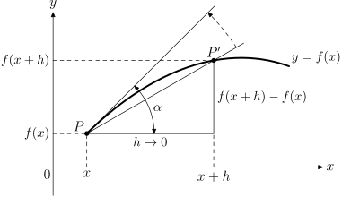
A quintessentially analytic property is the derivative of a (real-valued) function. The concept of derivative is first suggested by the intuitive notion of the tangent to a smooth curve $y = f(x)$ at a point $P$ with the coordinates $x$ and $y$. See Figure 6.3.1 for an illustration of this differentiation process. Mathematically, one shall generally use either the notation of Lagrange, $y' = f'(x)$, to denote the derivative, or, as Leibnitz did, the symbol $dy/dx$ or $df(x)/dx$. The notation $f'(x)$ indicates the fact that the derivative is itself a function of $x$ since a value of $f'(x)$ corresponds to each value of $x$ (in the interval considered). The definition of the derivative appears in several different forms, one of the following:
$$f'(x) = \lim_{h\rightarrow 0}\frac{f(x+h) - f(x)}{h}$$
One might expect to find a higher-order ‘derivative’ function deriv
$\colon (\mathbb{R}\rightarrow\mathbb{R})\rightarrow(\mathbb{R}\rightarrow\mathbb{R})$
mapping a function $f$ to its derivative $f'$. Actually, no such
thing is defined in HOL, but rather a ternary operator diffl
(defined in limTheory) where (f diffl l) x means 'the function $f$
has a derivative with value $l$ at the point $x$'. Expanding out the
definition, we see that the definition is much as an analyst might
expect:
diffl
  ⊢ ∀f l x. (f diffl l) x ⇔ ((λh. (f (x + h) − f x) / h) -> l) 0
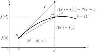
(f diffl l) x(f has_derivative f') (at x) means 'the function $f$ has a derivative
$f'$ at the point $x$', or (f has_derivative f') (at x within s) means
'the function $f$ has a derivative $f'$ at the point $x$ within the set
$s$'. Expanding out the definition, we see that the definition is much
as an analyst might expect: (cf. Figure 6.3.1 for an
illustration of this differentiation process.)
HAS_DERIVATIVE_AT
  ⊢ ∀f f' x.
       (f has_derivative f') (at x) ⇔
       linear f' ∧
       ∀e. 0 < e ⇒
           ∃d. 0 < d ∧
               ∀x'.
                 0 < abs (x' − x) ∧ abs (x' − x) < d ⇒
                 abs (f x' − f x − f' (x' − x)) / abs (x' − x) < e
f has_derivative f'has_vector_derivative
⊢ ∀f f' net.
(f has_vector_derivative f') net ⇔ (f has_derivative (λx. x * f')) net
Similarly, (f has_vector_derivative f') (at x) means that the function
$f$ has a derivative with value $f'$ at the point $x$. The usual kinds
of combining theorems are proved. For example, the derivative of a sum
of two functions is the sum of their derivatives:
DIFF_ADD
  ⊢ ∀f g l m x.
       (f diffl l) x ∧ (g diffl m) x ⇒ ((λx. f x + g x) diffl (l + m)) x

HAS_DERIVATIVE_ADD
  ⊢ ∀f f' g g' net.
       (f has_derivative f') net ∧ (g has_derivative g') net ⇒
       ((λx. f x + g x) has_derivative (λh. f' h + g' h)) net

DIFF_MUL
  ⊢ ∀f g l m x.
       (f diffl l) x ∧ (g diffl m) x ⇒
       ((λx. f x * g x) diffl (l * g x + m * f x)) x

HAS_DERIVATIVE_MUL_AT
  ⊢ ∀f f' g g' a.
       (f has_derivative f') (at a) ∧ (g has_derivative g') (at a) ⇒
       ((λx. f x * g x) has_derivative (λh. f a * g' h + f' h * g a)) (at a)

DIFF_DIV
  ⊢ ∀f g l m x.
       (f diffl l) x ∧ (g diffl m) x ∧ g x ≠ 0 ⇒
       ((λx. f x / g x) diffl ((l * g x − m * f x) / (g x)²)) x

DIFF_CHAIN
  ⊢ ∀f g l m x.
       (f diffl l) (g x) ∧ (g diffl m) x ⇒ ((λx. f (g x)) diffl (l * m)) x

limTheory.MVT
  ⊢ ∀f a b.
       a < b ∧ (∀x. a ≤ x ∧ x ≤ b ⇒ f contl x) ∧
       (∀x. a < x ∧ x < b ⇒ f differentiable x) ⇒
       ∃l z. a < z ∧ z < b ∧ (f diffl l) z ∧ f b − f a = (b − a) * l

derivativeTheory.MVT
  ⊢ ∀f f' a b.
       a < b ∧ f continuous_on interval [(a,b)] ∧
       (∀x. x ∈ interval (a,b) ⇒ (f has_derivative f' x) (at x)) ⇒
       ∃x. x ∈ interval (a,b) ∧ f b − f a = f' x (b − a)

diffl_has_vector_derivative
  ⊢ ∀f l x. (f diffl l) x ⇔ (f has_vector_derivative l) (at x)
A function is differentiable at certain point if it has derivative at that point.
The continuity of a function is very close with its differentiability.
The HOL formalization of "$f$ is (right-)continuous at the point $x$"
is f contl x with contl ('locally continuous' from limTheory),
or f continuous (at x) from real_topologyTheory, both are infix
binary operators. The two operators are equivalent (when continuous
is used with the at net) by the following bridging theorem:
contl_eq_continuous_at
  ⊢ ∀f x. f contl x ⇔ f continuous at x
However, using continuous it is also possible to express continuity
of a function at a point within a set of points (usually an
interval), i.e. f continuous (at x within s).
The global version of continuous for a set of points (usually an
open or closed interval) is called continuous_on.4
continuous_on
  ⊢ ∀f s.
       f continuous_on s ⇔
       ∀x. x ∈ s ⇒
           ∀e. 0 < e ⇒
               ∃d. 0 < d ∧
                   ∀x'. x' ∈ s ∧ dist (x',x) < d ⇒ dist (f x',f x) < e

CONTINUOUS_ON_EQ_CONTINUOUS_AT
  ⊢ ∀f s. open s ⇒ (f continuous_on s ⇔ ∀x. x ∈ s ⇒ f continuous at x)

CONTINUOUS_ON_EQ_CONTINUOUS_WITHIN
  ⊢ ∀f s. f continuous_on s ⇔ ∀x. x ∈ s ⇒ f continuous (at x within s)
One of the most fundamental facts about continuous functions is the intermediate value property (IVT): if a function takes two values then it also somewhere takes any value in between. The HOL formulation is that if $f$ is continuous at all points of an interval $[a,b]$, and $f(a)\leqslant y\leqslant f(b)$ then there is some point $x$ in the interval where $f(x) = y$:
IVT
  ⊢ ∀f a b y.
       a ≤ b ∧ (f a ≤ y ∧ y ≤ f b) ∧ (∀x. a ≤ x ∧ x ≤ b ⇒ f contl x) ⇒
       ∃x. a ≤ x ∧ x ≤ b ∧ f x = y

CONTINUOUS_ON_IVT
  ⊢ ∀f a b y.
       a ≤ b ∧ f a ≤ y ∧ y ≤ f b ∧ f continuous_on interval [(a,b)] ⇒
       ∃x. x ∈ interval [(a,b)] ∧ f x = y

IVT2
  ⊢ ∀f a b y.
       a ≤ b ∧ (f b ≤ y ∧ y ≤ f a) ∧ (∀x. a ≤ x ∧ x ≤ b ⇒ f contl x) ⇒
       ∃x. a ≤ x ∧ x ≤ b ∧ f x = y
Integration
The version of integral calculus formalized in HOL is a generalized Riemann integration called Henstock-Kurzweil Integration, or gauge integration (Bartle 2001). Many functions which are not Riemann integrable can be shown to be Henstock-Kurzweil integrable. (In particular, a function is Lebesgue integrable if and only if the function and its absolute value are Henstock-Kurzweil integrable.)
f integrable_on s means that the function $f$ is integrable on a
real set $s$ (there is another similar concept called absolute
integrability: f absolutely_integrable_on s.) If $f$ is integrable
on a closed interval $[a,b]$, then the usual integration of $f$ on
$[a,b]$, i.e. $\displaystyle\int_a^b f \,\mathrm{d}x$, is denoted by
integral (interval [a,b]) f in HOL. In general, the integration of
$f$ on a set $s$ of real numbers is integral s f.
gauge
  ⊢ ∀E g. gauge E g ⇔ ∀x. E x ⇒ 0 < g x

fine
  ⊢ ∀g D p. fine g (D,p) ⇔ ∀n. n < dsize D ⇒ D (SUC n) − D n < g (p n)

tdiv
  ⊢ ∀a b D p.
       tdiv (a,b) (D,p) ⇔ division (a,b) D ∧ ∀n. D n ≤ p n ∧ p n ≤ D (SUC n)

division
  ⊢ ∀a b D.
       division (a,b) D ⇔
       D 0 = a ∧ ∃N. (∀n. n < N ⇒ D n < D (SUC n)) ∧ ∀n. n ≥ N ⇒ D n = b

Dint
  ⊢ ∀a b f k.
       Dint (a,b) f k ⇔
       ∀e. 0 < e ⇒
           ∃g. gauge (λx. a ≤ x ∧ x ≤ b) g ∧
               ∀D p.
                 tdiv (a,b) (D,p) ∧ fine g (D,p) ⇒ abs (rsum (D,p) f − k) < e

integral
  ⊢ ∀a b f. integral (a,b) f = @i. Dint (a,b) f i
In integration, ported from HOL Light, a more general form of
Henstock-Kurzweil integration has been defined:
gauge_def
  ⊢ ∀d. gauge d ⇔ ∀x. x ∈ d x ∧ open (d x)

FINE
  ⊢ ∀d s. d FINE s ⇔ ∀x k. (x,k) ∈ s ⇒ k ⊆ d x

tagged_partial_division_of
  ⊢ ∀s i.
       s tagged_partial_division_of i ⇔
       FINITE s ∧
       (∀x k. (x,k) ∈ s ⇒ x ∈ k ∧ k ⊆ i ∧ ∃a b. k = interval [(a,b)]) ∧
       ∀x1 k1 x2 k2.
         (x1,k1) ∈ s ∧ (x2,k2) ∈ s ∧ (x1,k1) ≠ (x2,k2) ⇒
         interior k1 ∩ interior k2 = ∅

tagged_division_of
  ⊢ ∀s i.
       s tagged_division_of i ⇔
       s tagged_partial_division_of i ∧ BIGUNION {k | (∃x. (x,k) ∈ s)} = i

has_integral_compact_interval
  ⊢ ∀f y i.
       (f has_integral_compact_interval y) i ⇔
       ∀e. 0 < e ⇒
           ∃d. gauge d ∧
               ∀p. p tagged_division_of i ∧ d FINE p ⇒
                   abs (sum p (λ(x,k). content k * f x) − y) < e

has_integral_def
  ⊢ ∀f y i.
       (f has_integral y) i ⇔
       if ∃a b. i = interval [(a,b)] then
         (f has_integral_compact_interval y) i
       else
         ∀e. 0 < e ⇒
             ∃B. 0 < B ∧
                 ∀a b.
                   ball (0,B) ⊆ interval [(a,b)] ⇒
                   ∃z. ((λx. if x ∈ i then f x else 0) has_integral_compact_interval
                        z) (interval [(a,b)]) ∧ abs (z − y) < e

integral_def
  ⊢ ∀i f. integral i f = @y. (f has_integral y) i
The fundamental theorem of calculus (in the equivalent forms of Riemann integral) is expressed below:
FTC1
  ⊢ ∀f f' a b.
       a ≤ b ∧ (∀x. a ≤ x ∧ x ≤ b ⇒ (f diffl f' x) x) ⇒
       Dint (a,b) f' (f b − f a)

FUNDAMENTAL_THEOREM_OF_CALCULUS
  ⊢ ∀f f' a b.
       a ≤ b ∧
       (∀x. x ∈ interval [(a,b)] ⇒
            (f has_vector_derivative f' x) (at x within interval [(a,b)])) ⇒
       (f' has_integral f b − f a) (interval [(a,b)])
The above theorem requires that the function $f$ must be everywhere differentiable (i.e., has derivative) in the closed interval $[a,b]$. In fact, Henstock-Kurzweil Integration permits a countable number of exceptional points. This yields a significant improvement, as shown in the following strong version of the fundamental theorem of calculus:
FUNDAMENTAL_THEOREM_OF_CALCULUS_STRONG
  ⊢ ∀f f' s a b.
       countable s ∧ a ≤ b ∧ f continuous_on interval [(a,b)] ∧
       (∀x. x ∈ interval [(a,b)] DIFF s ⇒
            (f has_vector_derivative f' x) (at x within interval [(a,b)])) ⇒
       (f' has_integral f b − f a) (interval [(a,b)])
Finally, the following two bridging theorems can be used to convert
between integrals of the integral and integration theories:
integral_old_to_new
  ⊢ ∀f a b.
       a ≤ b ∧ integrable (a,b) f ⇒
       integral (a,b) f = integral (interval [(a,b)]) f

integral_new_to_old
  ⊢ ∀f a b.
       a ≤ b ∧ f integrable_on interval [(a,b)] ⇒
       integral (interval [(a,b)]) f = integral (a,b) f
Measure Theory
The theme of measure theory implemented in sigma_algebra and
measure theories is the problem of how to assign a size, a content,
a probability, etc. to certain sets. The most common examples of
measure is the length (in one dimension), area (in two dimensions)
and volume (in three dimensions) in Euclidean spaces. In HOL's
measure theory, a measure is a set function of the type $(\alpha
\to \konst{bool}) \to \konst{extreal}$.5 (See
Section 5.3.7 for more details of extended real numbers.)
This allows us to express, for example, the “length” of the entire
real line $\mathbb{R}$, i.e. PosInf.
A reasonable measure should be able to deal with disjoint countable
partitions of sets. Therefore a measure function must be defined on
a system of sets which is stable whenever we repeat any of the basic
set operations -- $\cup$, $\cap$, ${}^{\mathrm{c}}$ -- countably many
times, i.e. $\sigma$-algebra. In HOL, a system of sets is a pair
(sp,sts) of the type $(\alpha \to \konst{bool}) \,\#\, ((\alpha \to
\konst{bool}) \to \konst{bool})$ satisfying subset_class sp sts:
subset_class_def
  ⊢ ∀sp sts. subset_class sp sts ⇔ ∀x. x ∈ sts ⇒ x ⊆ sp
Given any system of sets a = (sp,sts), the two functions space
and subsets can be used to access sp and sts, respectively.
Then algebra and $\sigma$-algebra6 are defined below:
algebra_def
  ⊢ ∀a. algebra a ⇔
         subset_class (space a) (subsets a) ∧ ∅ ∈ subsets a ∧
         (∀s. s ∈ subsets a ⇒ space a DIFF s ∈ subsets a) ∧
         ∀s t. s ∈ subsets a ∧ t ∈ subsets a ⇒ s ∪ t ∈ subsets a

sigma_algebra_def
  ⊢ ∀a. sigma_algebra a ⇔
         algebra a ∧ ∀c. countable c ∧ c ⊆ subsets a ⇒ BIGUNION c ∈ subsets a
There are several equivalent ways of defining $\sigma$-algebra. The following alternative definition (as a theorem), for instance, perfectly matches Definition 3.1 of (Schilling 2017):
SIGMA_ALGEBRA_ALT_SPACE
  ⊢ ∀a. sigma_algebra a ⇔
         subset_class (space a) (subsets a) ∧ space a ∈ subsets a ∧
         (∀s. s ∈ subsets a ⇒ space a DIFF s ∈ subsets a) ∧
         ∀f. f ∈ (𝕌(:num) → subsets a) ⇒
             BIGUNION (IMAGE f 𝕌(:num)) ∈ subsets a
Any measure (function) must be defined with respect to a measure
space. In HOL, a measure space is represented by a tuple
(sp,sts,mu), where sp and sts forms a
$\sigma$-algebra7, and mu is the measure
function. If m = (sp,sts,mu) is a measure space, the functions
m_space, measurable_sets and measure can be used to access
sp, sts and mu, respectively. Any measure space must be both
positive and countably_additive:
measure_space_def
  ⊢ ∀m. measure_space m ⇔
         sigma_algebra (measurable_space m) ∧ positive m ∧
         countably_additive m

positive_def
  ⊢ ∀m. positive m ⇔
         measure m ∅ = 0 ∧ ∀s. s ∈ measurable_sets m ⇒ 0 ≤ measure m s

countably_additive_def
  ⊢ ∀m. countably_additive m ⇔
         ∀f. f ∈ (𝕌(:num) → measurable_sets m) ∧
             (∀i j. i ≠ j ⇒ DISJOINT (f i) (f j)) ∧
             BIGUNION (IMAGE f 𝕌(:num)) ∈ measurable_sets m ⇒
             measure m (BIGUNION (IMAGE f 𝕌(:num))) = suminf (measure m ∘ f)
In particular, if (sp,sts,mu) is positive and
countably_additive but (sp,sts) is not (yet) a $\sigma$-algebra,
it is called a premeasure (space):
premeasure_def
  ⊢ ∀m. premeasure m ⇔ positive m ∧ countably_additive m
The reason of introducing premeasure is that it is not a trivial task to assign explicitly a value to every set from a $\sigma$-algebra. Rather than doing this it is often more natural to assign values to sets from some generators. To get such an automatic extension the following (technically motivated) class of generators is useful. A semiring (usually denoted by $\mathscr{S}$) is a family with the following properties:
sigma_algebraTheory.semiring_def
  ⊢ ∀r. semiring r ⇔
         subset_class (space r) (subsets r) ∧ ∅ ∈ subsets r ∧
         (∀s t. s ∈ subsets r ∧ t ∈ subsets r ⇒ s ∩ t ∈ subsets r) ∧
         ∀s t.
           s ∈ subsets r ∧ t ∈ subsets r ⇒
           ∃c. c ⊆ subsets r ∧ FINITE c ∧ disjoint c ∧ s DIFF t = BIGUNION c
Any ($\sigma$-)algebra is also a semiring but not vice versa. For
instance, the set of all right open intervals $\big\{ [a,b) \colon
a,b\in\mathbb{R} \big\}$ is a semiring (because the set difference of
any two right open intervals is at most two new right open
intervals). Furthermore, for any system of sets (sp sts) there
exists a smallest $\sigma$-algebra containing it (also called the
$\sigma$-algebra generated from it), denoted by $\sigma(\cdot)$:
sigma_def
  ⊢ ∀sp sts.
       sigma sp sts = (sp,BIGINTER {s | sts ⊆ s ∧ sigma_algebra (sp,s)})

SIGMA_ALGEBRA_SIGMA
  ⊢ ∀sp sts. subset_class sp sts ⇒ sigma_algebra (sigma sp sts)

SIGMA_SUBSET_SUBSETS
  ⊢ ∀sp a. a ⊆ subsets (sigma sp a)
The following deep extension theorem for measures goes back to Carathéodory (Schilling 2017):
CARATHEODORY_SEMIRING
  ⊢ ∀m0.
       semiring (measurable_space m0) ∧ premeasure m0 ⇒
       ∃m. (∀s. s ∈ measurable_sets m0 ⇒ measure m s = measure m0 s) ∧
           measurable_space m = sigma (m_space m0) (measurable_sets m0) ∧
           measure_space m
In addition, the uniqueness of measures extended from generators is guaranteed by the following theorem, given that the involved generators are stable under $\cap$ and $\sigma$-finite:
sigma_finite_def
  ⊢ ∀m. sigma_finite m ⇔
         ∃f. f ∈ (𝕌(:num) → measurable_sets m) ∧ (∀n. f n ⊆ f (SUC n)) ∧
             BIGUNION (IMAGE f 𝕌(:num)) = m_space m ∧
             ∀n. measure m (f n) < +∞

sigma_finite_measure_space_def
  ⊢ ∀m. sigma_finite_measure_space m ⇔ measure_space m ∧ sigma_finite m

UNIQUENESS_OF_MEASURE
  ⊢ ∀sp sts u v.
       subset_class sp sts ∧ (∀s t. s ∈ sts ∧ t ∈ sts ⇒ s ∩ t ∈ sts) ∧
       sigma_finite (sp,sts,u) ∧
       measure_space (sp,subsets (sigma sp sts),u) ∧
       measure_space (sp,subsets (sigma sp sts),v) ∧
       (∀s. s ∈ sts ⇒ u s = v s) ⇒
       ∀s. s ∈ subsets (sigma sp sts) ⇒ u s = v s
Borel measurable function and sets
The theory real_borel provides Borel sets and Borel measurable
functions based on reals, in addition the theory borel provides the
same things based on extreals, plus the constructions of Borel and
Lebesgue measure spaces.
In HOL, the real-valued Borel sets borel $\mathscr{B}(\mathbb{R})$
is the $\sigma$-algebra generated by open sets (of the type
$\konst{real} \to \konst{bool}$).
borel
  ⊢ borel = sigma 𝕌(:real) {s | open s}
borel can also be generated by half spaces, open or closed
intervals:
borel_eq_le
  ⊢ borel = sigma 𝕌(:real) (IMAGE (λa. {x | x ≤ a}) 𝕌(:real))
borel_eq_less
  ⊢ borel = sigma 𝕌(:real) (IMAGE (λa. {x | x < a}) 𝕌(:real))
borel_eq_gr
  ⊢ borel = sigma 𝕌(:real) (IMAGE (λa. {x | a < x}) 𝕌(:real))
borel_eq_gr_le
  ⊢ borel =
     sigma 𝕌(:real) (IMAGE (λ(a,b). {x | a < x ∧ x ≤ b}) 𝕌(:real # real))
borel_eq_gr_less
  ⊢ borel =
     sigma 𝕌(:real) (IMAGE (λ(a,b). {x | a < x ∧ x < b}) 𝕌(:real # real))
borel_eq_ge_le
  ⊢ borel =
     sigma 𝕌(:real) (IMAGE (λ(a,b). {x | a ≤ x ∧ x ≤ b}) 𝕌(:real # real))
borel_eq_ge_less
  ⊢ borel =
     sigma 𝕌(:real) (IMAGE (λ(a,b). {x | a ≤ x ∧ x < b}) 𝕌(:real # real))
The extreal-valued Borel sets Borel
$\mathscr{B}(\mathbb{\overline{R}})$ is defined by augmenting borel
with infinities:
Borel
  ⊢ Borel =
     (𝕌(:extreal),
      {B' |
       ∃B S.
         B' = IMAGE Normal B ∪ S ∧ B ∈ subsets borel ∧
         S ∈ {∅; {−∞}; {+∞}; {−∞; +∞}}})
Borel can also be generated by half spaces (of the type
$\konst{extreal} \to \konst{bool}$):8
Borel_def
  ⊢ Borel = sigma 𝕌(:extreal) (IMAGE (λa. {x | x < Normal a}) 𝕌(:real))
Borel_eq_le
  ⊢ Borel = sigma 𝕌(:extreal) (IMAGE (λa. {x | x ≤ Normal a}) 𝕌(:real))
Borel_eq_gr
  ⊢ Borel = sigma 𝕌(:extreal) (IMAGE (λa. {x | Normal a < x}) 𝕌(:real))
Borel_eq_ge
  ⊢ Borel = sigma 𝕌(:extreal) (IMAGE (λa. {x | Normal a ≤ x}) 𝕌(:real))
Let a and b be two measurable spaces ($\sigma$-algebras). A map
$f \colon \konst{space}\,a \to \konst{space}\,b$ is called
$a/b$-measurable (or measurable unless this is too ambiguous) if
the pre-image of every measurable set is a measurable set: (the
definition is in sigma_algebra theory)
measurable_def
  ⊢ ∀a b.
       measurable a b =
       {f |
        f ∈ (space a → space b) ∧
        ∀s. s ∈ subsets b ⇒ PREIMAGE f s ∩ space a ∈ subsets a}
A function is called Borel-measurable if it is a measurable map
from any measurable space to borel or Borel:
val _ = overload_on ("borel_measurable", ``\a. measurable a borel``);
val _ = overload_on ("Borel_measurable", ``\a. measurable a Borel``);
For instance, a random variable is nothing but a measurable map from
a probability space (which is also a measure space, see Section
6.6) to Borel. Thus in HOL there are actually two
different types of Borel-measurable functions, real-valued or
extreal-valued, each with a large set of theorems for proving the
Borel-measurabilities, in real_borel and borel theories,
respectively. For instance, the addition or subtraction of two
real-valued (or extreal-valued) Borel-measurable functions $f$ and
$g$ is still Borel-measurable:
in_borel_measurable_add
  ⊢ ∀a f g h.
       sigma_algebra a ∧ f ∈ borel_measurable a ∧ g ∈ borel_measurable a ∧
       (∀x. x ∈ space a ⇒ h x = f x + g x) ⇒
       h ∈ borel_measurable a

IN_MEASURABLE_BOREL_ADD'
  ⊢ ∀a f g h.
       sigma_algebra a ∧ f ∈ Borel_measurable a ∧ g ∈ Borel_measurable a ∧
       (∀x. x ∈ space a ⇒ h x = f x + g x) ⇒
       h ∈ Borel_measurable a

in_borel_measurable_sub
  ⊢ ∀a f g h.
       sigma_algebra a ∧ f ∈ borel_measurable a ∧ g ∈ borel_measurable a ∧
       (∀x. x ∈ space a ⇒ h x = f x − g x) ⇒
       h ∈ borel_measurable a

IN_MEASURABLE_BOREL_SUB'
  ⊢ ∀a f g h.
       sigma_algebra a ∧ f ∈ Borel_measurable a ∧ g ∈ Borel_measurable a ∧
       (∀x. x ∈ space a ⇒ h x = f x − g x) ⇒
       h ∈ Borel_measurable a

in_borel_measurable_mul
  ⊢ ∀a f g h.
       sigma_algebra a ∧ f ∈ borel_measurable a ∧ g ∈ borel_measurable a ∧
       (∀x. x ∈ space a ⇒ h x = f x * g x) ⇒
       h ∈ borel_measurable a

IN_MEASURABLE_BOREL_TIMES'
  ⊢ ∀a f g h.
       sigma_algebra a ∧ f ∈ Borel_measurable a ∧ g ∈ Borel_measurable a ∧
       (∀x. x ∈ space a ⇒ h x = f x * g x) ⇒
       h ∈ Borel_measurable a
Furthermore, if a real-valued function is Borel-measurable, so is its extreal-valued version. The converse also holds.
IN_MEASURABLE_BOREL_IMP_BOREL'
  ⊢ ∀a f.
       sigma_algebra a ∧ f ∈ borel_measurable a ⇒
       Normal ∘ f ∈ Borel_measurable a

in_borel_measurable_from_Borel
  ⊢ ∀a f.
       sigma_algebra a ∧ f ∈ Borel_measurable a ⇒
       real ∘ f ∈ borel_measurable a
Construction of Borel measure space (lborel)
The Borel measure space lborel (of the type $(\konst{real} \to
\konst{bool}) \,\#\, ((\konst{real} \to \konst{bool}) \to
\konst{bool}) \,\#\, ((\konst{real} \to \konst{bool}) \to
\konst{extreal})$) is the household measure space defined on the
real-valued Borel sets (borel) such that any interval with end
points $a,b \in \mathbb{R}$ ($a \leqslant b$) has the extreal-valued
measure of $b - a \in \mathbb{\overline{R}}$. The construction of
lborel is done by extending a premeasure in the following steps:
-
Define the system of all right-open intervals and a “premeasure”
lambda0on it:right_open_interval ⊢ ∀a b. right_open_interval a b = {x | a ≤ x ∧ x < b} right_open_intervals ⊢ right_open_intervals = (𝕌(:real),{right_open_interval a b | T}) lambda0_def ⊢ ∀a b. a ≤ b ⇒ lambda0 (right_open_interval a b) = Normal (b − a) -
Prove that the set of all right open intervals is a semiring and the $\sigma$-algebra generated from it is nothing but
borel:right_open_intervals_semiring ⊢ semiring right_open_intervals right_open_intervals_sigma_borel ⊢ sigma (space right_open_intervals) (subsets right_open_intervals) = borel -
Prove
(space right_open_intervals, subsets right_open_intervals, lambda0)(abbreviated aslborel0) isadditive,finite_additiveand eventually apremeasure(positiveandcountably_additive):lborel0_additive ⊢ additive lborel0 lborel0_finite_additive ⊢ finite_additive lborel0 lborel0_premeasure ⊢ premeasure lborel0(The proof of
lborel0_premeasuredepends onreal_topologytheory, especially the Heine-Borel Theorem. See Section 6.2.) -
By Carathéodory Extension Theorem (
CARATHEODORY_SEMIRING, see Section 6.4), there exists an extension oflborel0, denoted bylborel, which is now a measure space:lborel_def ⊢ (∀s. s ∈ subsets right_open_intervals ⇒ lambda s = lambda0 s) ∧ measurable_space lborel = borel ∧ measure_space lborel
Let lambda = measure lborel be an abbreviation, the measure of the
following typical Borel sets are proved as theorems:
lambda_prop
  ⊢ ∀a b. a ≤ b ⇒ lambda (right_open_interval a b) = Normal (b − a)

lambda_sing
  ⊢ ∀c. lambda {c} = 0

lambda_open_interval
  ⊢ ∀a b. a ≤ b ⇒ lambda (interval (a,b)) = Normal (b − a)

lambda_closed_interval
  ⊢ ∀a b. a ≤ b ⇒ lambda (interval [(a,b)]) = Normal (b − a)
Furthermore, the extreal-based Borel measurable space (ext_lborel)
is defined by:
ext_lborel_def
  ⊢ ext_lborel = (space Borel,subsets Borel,lambda ∘ real_set)

real_set_def
  ⊢ ∀s. real_set s = {real x | x ≠ +∞ ∧ x ≠ −∞ ∧ x ∈ s}
where real_set (extreal theory) converts a set of extreals to
the corresponding set of reals, filtering out $\pm\infty$. It can be
proven that ext_lborel is indeed a $\sigma$-finite measure space:
measure_space_ext_lborel
  ⊢ measure_space ext_lborel

sigma_finite_ext_lborel
  ⊢ sigma_finite ext_lborel
Construction of Lebesgue measure space (lebesgue)
It is well known that lborel is not complete, in the sense that
if for non-empty set s we have lambda s = 0, it's not true that
all subsets of s has also the measure 0, as some of them may not be
Borel sets at all. The completion of lborel is called Lebesgue
measure space, denoted by lebesgue. In extreal theory (at
$(HOLDIR)/examples/probability directory), it is defined directly
by Henstock-Kurzweil Integration (see Section 6.3.2):
lebesgue_def
  ⊢ lebesgue =
     (𝕌(:real),{A | ∀n. indicator A integrable_on line n},
      (λA. sup {Normal (integral (line n) (indicator A)) | n ∈ 𝕌(:num)}))

real_borelTheory.line
  ⊢ ∀n. line n = {x | -&n ≤ x ∧ x ≤ &n}
The above definition indeed defines a $\sigma$-algebra and measure
space. The Lebesgue measure of closed intervals is also proven
(directly by integration theory):
sigma_algebra_lebesgue
  ⊢ sigma_algebra (𝕌(:real),{A | ∀n. indicator A integrable_on line n})

measure_space_lebesgue
  ⊢ measure_space lebesgue

lebesgue_closed_interval
  ⊢ ∀a b. a ≤ b ⇒ lmeasure (interval [(a,b)]) = Normal (b − a)
Now comes the relationship between lborel and lebesgue, which
have two very different definitions. In fact, all
Borel-measurable sets are also Lebesgue-measurable sets:
borel_imp_lebesgue_sets
  ⊢ ∀s. s ∈ subsets borel ⇒ s ∈ measurable_sets lebesgue
Finally, by uniqueness of measure, the two measure spaces lborel
and lebesgue coincide on Borel sets (recall that lambda is an
abbreviation of measure lborel):
lebesgue_eq_lambda
  ⊢ ∀s. s ∈ subsets borel ⇒ lmeasure s = lambda s
Lebesgue Integration Theory
The fundamental idea of integration is to measure the area between the graph of a function and the abscissa (i.e. $x$-axis). Riemann's approach partitions the domain of the function without taking into account the shape of the function, thus slicing up the area under the function vertically. Lebesgue's approach is exactly the opposite: the domain is partitioned according to the values of the function at hand, leading to a horizontal decomposition of the area.
In case the values of the function $f$ is finite, its domain can also be decomposed into the same number of disjoint sets (but each of them may not be a continuous interval). If the function is also nonnegative, i.e. $\forall x.\,0 \leqslant f(x)$, this function is called a positive simple function which can be also represented by a finite sum:
$$f = \sum_{j=0}^M y_j \mathbf{1}_{A_j}, \quad \text{where $\forall x\in A_j.\,f(x) = y_j$.}\quad\quad (\text{eq:posSimpleFn})$$
And the “integration” of $f$ is simply $\sum_{j=0}^M y_j\mu(A_j)$,
where $\mu$ is the measure function of a measure space, e.g.
lborel and lebesgue constructed in Section 6.4.1.
Note that the representations of positive simple functions are not
unique, but each representation can be uniquely determined by an
index set $J$, a disjoint set of sets $A_j, j \in J$ and the set of
values $y_j$ corresponding to each $A_j$. In HOL, the connection
between positive simple functions (extreal-valued) and their
representations is captured by pos_simple_fn, while the integration
of positive simple functions is defined by pos_simple_fn_integral:
pos_simple_fn_def
  ⊢ ∀m f s a x.
       pos_simple_fn m f s a x ⇔
       (∀t. t ∈ m_space m ⇒ 0 ≤ f t) ∧
       (∀t. t ∈ m_space m ⇒ f t = ∑ (λi. Normal (x i) * 𝟙 (a i) t) s) ∧
       (∀i. i ∈ s ⇒ a i ∈ measurable_sets m) ∧ FINITE s ∧
       (∀i. i ∈ s ⇒ 0 ≤ x i) ∧
       (∀i j. i ∈ s ∧ j ∈ s ∧ i ≠ j ⇒ DISJOINT (a i) (a j)) ∧
       BIGUNION (IMAGE a s) = m_space m

pos_simple_fn_integral_def
  ⊢ ∀m s a x.
       pos_simple_fn_integral m s a x =
       ∑ (λi. Normal (x i) * measure m (a i)) s
Since the representations of a positive simple function are not
unique, for each positive simple function there exists a set of
representations (psfs), and a set of integrations (psfis)
(although it can be proved that all these integrations are the
same). The integration of an arbitrary positive function $f$ is
defined as the supremum of all positive simple functions $g$ which is
pointwise smaller than $f$:
pos_fn_integral_def
  ⊢ ∀m f.
       ∫⁺ m f = sup {r | (∃g. r ∈ psfis m g ∧ ∀x. x ∈ m_space m ⇒ g x ≤ f x)}

psfs_def
  ⊢ ∀m f. psfs m f = {(s,a,x) | pos_simple_fn m f s a x}

psfis_def
  ⊢ ∀m f.
       psfis m f =
       IMAGE (λ(s,a,x). pos_simple_fn_integral m s a x) (psfs m f)
For any positive function $f$, it is possible to construct a pointwise increasing sequence of positive simple functions $f_i$ which is always pointwise smaller than $f$. In another words, each $f(x)$ is the limit of $f_i(x)$ which is mono-increasing with $i$. Then the following monotone convergence theorem (actually due to Beppo Levi, see (Schilling 2017, 75)) reduces the integration of $f$ to the limit of integrations of $f_i$:
lebesgue_monotone_convergence
  ⊢ ∀m f fi.
       measure_space m ∧ (∀i. fi i ∈ Borel_measurable (measurable_space m)) ∧
       (∀i x. x ∈ m_space m ⇒ 0 ≤ fi i x) ∧
       (∀x. x ∈ m_space m ⇒ mono_increasing (λi. fi i x)) ∧
       (∀x. x ∈ m_space m ⇒ sup (IMAGE (λi. fi i x) 𝕌(:num)) = f x) ⇒
       ∫⁺ m f = sup (IMAGE (λi. ∫⁺ m (fi i)) 𝕌(:num))
Finally, the (Lebesgue) integration of an arbitrary function $f$ is defined by the subtraction of integrations of its positive and negative parts:
integral_def
  ⊢ ∀m f. ∫ m f = ∫⁺ m f⁺ − ∫⁺ m f⁻

extrealTheory.fn_plus_def
  ⊢ ∀f. f⁺ = (λx. if 0 < f x then f x else 0)

extrealTheory.fn_minus_def
  ⊢ ∀f. f⁻ = (λx. if f x < 0 then -f x else 0)
Note that it is possible that the two integrations above both result
in the PosInf value, giving the entire integration an unspecified
value (see Section 5.3.7 for more details on extreal
arithmetics). A function $f$ is (Lebesgue) integrable if it is
Borel-measurable and the integrations of its positive and negative
parts are both finite (i.e. not $+\infty$):
integrable_def
  ⊢ ∀m f.
       integrable m f ⇔
       f ∈ Borel_measurable (measurable_space m) ∧ ∫⁺ m f⁺ ≠ +∞ ∧
       ∫⁺ m f⁻ ≠ +∞
A large set of theorems are provided in lebesgue theory on the
properties of integrable functions and their integrations, including
the following famous Markov's inequality:
markov_inequality
  ⊢ ∀m f a c.
       measure_space m ∧ integrable m f ∧ a ∈ measurable_sets m ∧ 0 < c ⇒
       measure m ({x | c ≤ abs (f x)} ∩ a) ≤
       c⁻¹ * ∫ m (λx. abs (f x) * 𝟙 a x)
Null sets and ‘almost everywhere’
A measurable set is called null set (with respect to its measure space) if its measure is zero:
null_set_def
  ⊢ ∀m s. null_set m s ⇔ s ∈ measurable_sets m ∧ measure m s = 0
A property $P(x)$ holds almost everywhere (AE) in a measure space
$m$, denoted by AE x::m. P x in HOL9, if
$P(x)$ holds for every $x$ excluding a null set:
borelTheory.AE_DEF
  ⊢ ∀m P. (AE x::m. P x) ⇔ ∃N. null_set m N ∧ ∀x. x ∈ m_space m DIFF N ⇒ P x
‘Almost everywhere’ is the basis of AE convergence in probability theory (see the next section). The following two theorems about the integration on null sets are very useful (Theorem 11.2 of (Schilling 2017, 89–90)):
integral_abs_eq_0
  ⊢ ∀m f.
       measure_space m ∧ f ∈ Borel_measurable (measurable_space m) ⇒
       (∫ m (abs ∘ f) = 0 ⇔ AE x::m. (abs ∘ f) x = 0) ∧
       ((AE x::m. (abs ∘ f) x = 0) ⇔
        measure m {x | x ∈ m_space m ∧ f x ≠ 0} = 0)

integral_null_set
  ⊢ ∀m f N.
       measure_space m ∧ f ∈ Borel_measurable (measurable_space m) ∧
       N ∈ null_set m ⇒
       integrable m (λx. f x * 𝟙 N x) ∧ ∫ m (λx. f x * 𝟙 N x) = 0
Radon-Nikodým theorem
So far there is no concept “derivative” being discussed. In Lebesgue integration, Radon-Nikodým (RN) Theorem (see, e.g., (Schilling 2017, 230) or (Fitzpatrick and Royden 2010, 382)) has the position of “Fundamental Theorem of Calculus” as in Riemann Integration. Recall in Lebesgue's theory one starts directly from the concept “integration” without defining “derivative” first. It is RN theorem which introduces the concept of “derivative” for Lebesgue integration and asserts its existence. The theorem says that for any $\sigma$-finite measure space $m$, if there is another measure $v$ absolutely continuous with respect to $m$, i.e. whenever any set $s$ has zero measure in measure space $m$ it also has same zero measure in $v$:
measure_absolutely_continuous_def
  ⊢ ∀v m. v ≪ m ⇔ ∀s. s ∈ measurable_sets m ∧ measure m s = 0 ⇒ v s = 0
Then there exists a nonnegative Borel-measurable function $f$ such that the (positive) integral of $f$ on any measurable set $s$ is exactly $v(s)$:
Radon_Nikodym
  ⊢ ∀m v.
       measure_space m ∧ sigma_finite m ∧
       measure_space (m_space m,measurable_sets m,v) ∧ v ≪ m ⇒
       ∃f. f ∈ Borel_measurable (measurable_space m) ∧ (∀x. 0 ≤ f x) ∧
           ∀s. s ∈ measurable_sets m ⇒ (f * m) s = v s

density_measure_def
  ⊢ ∀m f. f * m = (λs. ∫⁺ m (λx. f x * 𝟙 s x))
Given two such measures $m$ and $v$, The function $f$ asserted by RN theorem is called Radon-Nikodým derivative (denoted by $\displaystyle\frac{\mathrm{d}v}{\mathrm{d}m}$ in textbooks but overloaded on division in HOL):
RN_deriv_def
  ⊢ ∀v m.
       v / m =
       @f. f ∈ Borel_measurable (measurable_space m) ∧
           (∀x. x ∈ m_space m ⇒ 0 ≤ f x) ∧
           ∀s. s ∈ measurable_sets m ⇒ (f * m) s = v s
The overloading of * (density_measure) and / (RN_deriv) with
the particular argument order is to syntactically have
f * m / m = v / m = f.
Product measures and Fubini's theorem
HOL provides some basic support for (binary) products of measure
spaces (in martingale theory).
Let $(X,\mathcal{A},\mu)$ and $(Y,\mathcal{B},\nu)$ be two
$\sigma$-finite measure spaces, sometimes we want to define a measure
$\rho$ on rectangles of the form $A\times B$ such that
$\rho(A\times B) = \mu(A)\nu(B)$ for $A\in\mathcal{A}$ and
$B\in\mathcal{B}$. The first problem which we encounter is that
the family $\mathcal{A}\times\mathcal{B}$, denoted by prod_sets A B
(in sigma_algebra theory):
prod_sets_def
  ⊢ ∀a b. prod_sets a b = {s × t | s ∈ a ∧ t ∈ b}
is, in general, no $\sigma$-algebra — it contains only “rectangles”.
Definition. Let $(X,\mathcal{A})$ and $(Y,\mathcal{B})$ be two measurable spaces, then the $\sigma$-algebra $\mathcal{A}\otimes\mathcal{B} := \sigma(\mathcal{A}\times\mathcal{B})$ is called a product $\sigma$-algebra, and $(X\times Y,\mathcal{A}\otimes\mathcal{B})$ is the product of measurable spaces: ($\times$ is overloaded for $\otimes$ in HOL.)
sigma_algebraTheory.prod_sigma_def
  ⊢ ∀a b.
       a × b = sigma (space a × space b) (prod_sets (subsets a) (subsets b))
The following lemma is quite useful since it allows us to reduce considerations for $\mathcal{A}\otimes\mathcal{B}$ to generators $\mathcal{F}$ and $\mathcal{G}$ of $\mathcal{A}$ and $\mathcal{B}$:
PROD_SIGMA_OF_GENERATOR
  ⊢ ∀X Y E G.
       subset_class X E ∧ subset_class Y G ∧ has_exhausting_sequence (X,E) ∧
       has_exhausting_sequence (Y,G) ⇒
       (X,E) × (Y,G) = sigma X E × sigma Y G
The uniqueness and existence of product measures are guaranteed by the following theorems:
EXISTENCE_OF_PROD_MEASURE
  ⊢ ∀X Y A B u v m0.
       sigma_finite_measure_space (X,A,u) ∧
       sigma_finite_measure_space (Y,B,v) ∧
       (∀s t. s ∈ A ∧ t ∈ B ⇒ m0 (s × t) = u s * v t) ⇒
       (∀s. s ∈ subsets ((X,A) × (Y,B)) ⇒
            (∀x. x ∈ X ⇒ (λy. 𝟙 s (x,y)) ∈ Borel_measurable (Y,B)) ∧
            (∀y. y ∈ Y ⇒ (λx. 𝟙 s (x,y)) ∈ Borel_measurable (X,A)) ∧
            (λy. ∫⁺ (X,A,u) (λx. 𝟙 s (x,y))) ∈ Borel_measurable (Y,B) ∧
            (λx. ∫⁺ (Y,B,v) (λy. 𝟙 s (x,y))) ∈ Borel_measurable (X,A)) ∧
       ∃m. sigma_finite_measure_space (X × Y,subsets ((X,A) × (Y,B)),m) ∧
           (∀s. s ∈ prod_sets A B ⇒ m s = m0 s) ∧
           ∀s. s ∈ subsets ((X,A) × (Y,B)) ⇒
               m s = ∫⁺ (Y,B,v) (λy. ∫⁺ (X,A,u) (λx. 𝟙 s (x,y))) ∧
               m s = ∫⁺ (X,A,u) (λx. ∫⁺ (Y,B,v) (λy. 𝟙 s (x,y)))

UNIQUENESS_OF_PROD_MEASURE
  ⊢ ∀X Y E G A B u v m m'.
       subset_class X E ∧ subset_class Y G ∧ sigma_finite (X,E,u) ∧
       sigma_finite (Y,G,v) ∧ (∀s t. s ∈ E ∧ t ∈ E ⇒ s ∩ t ∈ E) ∧
       (∀s t. s ∈ G ∧ t ∈ G ⇒ s ∩ t ∈ G) ∧ A = sigma X E ∧ B = sigma Y G ∧
       measure_space (X,subsets A,u) ∧ measure_space (Y,subsets B,v) ∧
       measure_space (X × Y,subsets (A × B),m) ∧
       measure_space (X × Y,subsets (A × B),m') ∧
       (∀s t. s ∈ E ∧ t ∈ G ⇒ m (s × t) = u s * v t) ∧
       (∀s t. s ∈ E ∧ t ∈ G ⇒ m' (s × t) = u s * v t) ⇒
       ∀x. x ∈ subsets (A × B) ⇒ m x = m' x
Definition. Let $(X,\mathcal{A})$ and $(Y,\mathcal{B})$ be two
measurable spaces, the unique measure $\rho$ constructed in
EXISTENCE_OF_PROD_MEASURE is called the product of the measures
$\mu$ and $\nu$, denoted by $\mu\times\nu$.
$(X\times Y, \mathcal{A}\otimes\mathcal{B}, \mu\times\nu)$ is called
the product measure space:
prod_measure_def
  ⊢ ∀m1 m2. prod_measure m1 m2 = (λs. ∫⁺ m2 (λy. ∫⁺ m1 (λx. 𝟙 s (x,y))))
As an application, the two-dimensional (real-valued) Borel measure
space (lborel_2d) is constructed by the following definition and
theorem:
lborel_2d_def
  ⊢ sigma_finite_measure_space lborel_2d ∧
     m_space lborel_2d = 𝕌(:real) × 𝕌(:real) ∧
     measurable_sets lborel_2d =
     subsets ((𝕌(:real),subsets borel) × (𝕌(:real),subsets borel)) ∧
     (∀s t.
        s ∈ subsets borel ∧ t ∈ subsets borel ⇒
        measure lborel_2d (s × t) = lambda s * lambda t) ∧
     ∀s. s ∈ measurable_sets lborel_2d ⇒
         (∀x. (λy. 𝟙 s (x,y)) ∈ Borel_measurable borel) ∧
         (∀y. (λx. 𝟙 s (x,y)) ∈ Borel_measurable borel) ∧
         (λy. ∫⁺ lborel (λx. 𝟙 s (x,y))) ∈ Borel_measurable borel ∧
         (λx. ∫⁺ lborel (λy. 𝟙 s (x,y))) ∈ Borel_measurable borel ∧
         measure lborel_2d s = ∫⁺ lborel (λy. ∫⁺ lborel (λx. 𝟙 s (x,y))) ∧
         measure lborel_2d s = ∫⁺ lborel (λx. ∫⁺ lborel (λy. 𝟙 s (x,y)))

lborel_2d_prod_measure
  ⊢ ∀s. s ∈ measurable_sets lborel_2d ⇒
         measure lborel_2d s = measure (lborel × lborel) s
The next step is to see how we can integrate w.r.t. $\mu\times\nu$.
The following two results are often stated together as the Fubini
or Fubini-Tonelli theorem. Following (Schilling 2017), we
prefer to distinguish between them since the first result, TONELLI,
says that we can always swap iterated integrals of positive
functions (even if we get $+\infty$), whereas FUBINI applies to
more general functions but requires the (iterated) integrals to be
finite:
TONELLI
  ⊢ ∀X Y A B u v f.
       sigma_finite_measure_space (X,A,u) ∧
       sigma_finite_measure_space (Y,B,v) ∧
       f ∈ Borel_measurable ((X,A) × (Y,B)) ∧ (∀s. s ∈ X × Y ⇒ 0 ≤ f s) ⇒
       (∀y. y ∈ Y ⇒ (λx. f (x,y)) ∈ Borel_measurable (X,A)) ∧
       (∀x. x ∈ X ⇒ (λy. f (x,y)) ∈ Borel_measurable (Y,B)) ∧
       (λx. ∫⁺ (Y,B,v) (λy. f (x,y))) ∈ Borel_measurable (X,A) ∧
       (λy. ∫⁺ (X,A,u) (λx. f (x,y))) ∈ Borel_measurable (Y,B) ∧
       ∫⁺ ((X,A,u) × (Y,B,v)) f = ∫⁺ (Y,B,v) (λy. ∫⁺ (X,A,u) (λx. f (x,y))) ∧
       ∫⁺ ((X,A,u) × (Y,B,v)) f = ∫⁺ (X,A,u) (λx. ∫⁺ (Y,B,v) (λy. f (x,y)))

FUBINI
  ⊢ ∀X Y A B u v f.
       sigma_finite_measure_space (X,A,u) ∧
       sigma_finite_measure_space (Y,B,v) ∧
       f ∈ Borel_measurable ((X,A) × (Y,B)) ∧
       (∫⁺ ((X,A,u) × (Y,B,v)) (abs ∘ f) ≠ +∞ ∨
        ∫⁺ (Y,B,v) (λy. ∫⁺ (X,A,u) (λx. (abs ∘ f) (x,y))) ≠ +∞ ∨
        ∫⁺ (X,A,u) (λx. ∫⁺ (Y,B,v) (λy. (abs ∘ f) (x,y))) ≠ +∞) ⇒
       ∫⁺ ((X,A,u) × (Y,B,v)) (abs ∘ f) ≠ +∞ ∧
       ∫⁺ (Y,B,v) (λy. ∫⁺ (X,A,u) (λx. (abs ∘ f) (x,y))) ≠ +∞ ∧
       ∫⁺ (X,A,u) (λx. ∫⁺ (Y,B,v) (λy. (abs ∘ f) (x,y))) ≠ +∞ ∧
       integrable ((X,A,u) × (Y,B,v)) f ∧
       (AE y::(Y,B,v). integrable (X,A,u) (λx. f (x,y))) ∧
       (AE x::(X,A,u). integrable (Y,B,v) (λy. f (x,y))) ∧
       integrable (X,A,u) (λx. ∫ (Y,B,v) (λy. f (x,y))) ∧
       integrable (Y,B,v) (λy. ∫ (X,A,u) (λx. f (x,y))) ∧
       ∫ ((X,A,u) × (Y,B,v)) f = ∫ (Y,B,v) (λy. ∫ (X,A,u) (λx. f (x,y))) ∧
       ∫ ((X,A,u) × (Y,B,v)) f = ∫ (X,A,u) (λx. ∫ (Y,B,v) (λy. f (x,y)))
HOL also supports other types of “products”. In general, any three LISP-like pair operators can be used for building product measures:
pair_operation_def
  ⊢ ∀cons car cdr.
       pair_operation cons car cdr ⇔
       (∀a b. car (cons a b) = a ∧ cdr (cons a b) = b) ∧
       ∀a b c d. cons a b = cons c d ⇔ a = c ∧ b = d

pair_operation_pair
  ⊢ pair_operation $, FST SND
Besides pairTheory, one can also use FCP_CONCAT, FCP_FST and
FCP_SND (fcpTheory):
pair_operation_FCP_CONCAT
  ⊢ FINITE 𝕌(:β) ∧ FINITE 𝕌(:γ) ⇒ pair_operation FCP_CONCAT FCP_FST FCP_SND
The general version of product space is defined on any pair operation:
general_cross_def
  ⊢ ∀cons A B. general_cross cons A B = {cons a b | a ∈ A ∧ b ∈ B}

general_prod_def
  ⊢ ∀cons A B.
       general_prod cons A B = {general_cross cons a b | a ∈ A ∧ b ∈ B}
In fact, all the theorems about product measures, up to the
uniqueness and existence of product measures (i.e. except for
TONELLI and FUBINI), are first proven on general pair operations
(and then specialized on pairTheory and fcpTheory). For
instance, the following theorem is the general version of
EXISTENCE_OF_PROD_MEASURE:
existence_of_prod_measure_general
  ⊢ ∀cons car cdr X Y A B u v m0.
       pair_operation cons car cdr ∧ sigma_finite_measure_space (X,A,u) ∧
       sigma_finite_measure_space (Y,B,v) ∧
       (∀s t. s ∈ A ∧ t ∈ B ⇒ m0 (general_cross cons s t) = u s * v t) ⇒
       (∀s. s ∈ subsets (general_sigma cons (X,A) (Y,B)) ⇒
            (∀x. x ∈ X ⇒ (λy. 𝟙 s (cons x y)) ∈ Borel_measurable (Y,B)) ∧
            (∀y. y ∈ Y ⇒ (λx. 𝟙 s (cons x y)) ∈ Borel_measurable (X,A)) ∧
            (λy. ∫⁺ (X,A,u) (λx. 𝟙 s (cons x y))) ∈ Borel_measurable (Y,B) ∧
            (λx. ∫⁺ (Y,B,v) (λy. 𝟙 s (cons x y))) ∈ Borel_measurable (X,A)) ∧
       ∃m. sigma_finite_measure_space
             (general_cross cons X Y,
              subsets (general_sigma cons (X,A) (Y,B)),m) ∧
           (∀s. s ∈ general_prod cons A B ⇒ m s = m0 s) ∧
           ∀s. s ∈ subsets (general_sigma cons (X,A) (Y,B)) ⇒
               m s = ∫⁺ (Y,B,v) (λy. ∫⁺ (X,A,u) (λx. 𝟙 s (cons x y))) ∧
               m s = ∫⁺ (X,A,u) (λx. ∫⁺ (Y,B,v) (λy. 𝟙 s (cons x y)))
$\mathcal{L}^p$ spaces, semi-norm and important inequalities
HOL provides a minimal formalization of the function spaces
$\mathcal{L}^p$, currently in martingaleTheory.
Let $(X, \mathscr{A}, \mu)$ be some measure space. Here we discuss functions whose (absolute) $p$th power is integrable ($1\leqslant p <\infty$). More precisely, we are interested in the sets:
$$\mathcal{L}^p(\mu) := \left\{ u \colon X\rightarrow\overline{\mathbb{R}} \colon u\in\mathcal{M}(\mathscr{A}), \int |u|^p \,\mathrm{d}\mu < \infty \right\}, \qquad p\in[1,\infty).$$
Or formally:
lp_space_alt_finite
  ⊢ ∀p m f.
       0 < p ∧ p ≠ +∞ ⇒
       (f ∈ lp_space p m ⇔
        f ∈ Borel_measurable (measurable_space m) ∧
        ∫⁺ m (λx. abs (f x) powr p) ≠ +∞)
It is convenient to have the following semi-norm notation:
$$\|u\|_p := \left( \int \left|u(x)\right|^p \mu(\mathrm{d}x) \right)^{1/p}, \qquad p\in[1,\infty).$$
Or formally:
seminorm_normal
  ⊢ ∀p m f.
       0 < p ∧ p ≠ +∞ ⇒ seminorm p m f = ∫⁺ m (λx. abs (f x) powr p) powr p⁻¹
Clearly, $u\in\mathcal{L}^p(\mu)$ if, and only if, $u\in\mathcal{M}(\mathscr{A})$ and $\|u\|_p <\infty$. Furthermore, $\|u\|_p$ implies that $u(x) = 0$ for almost every $x$.
lp_space_alt_seminorm
  ⊢ ∀p m f.
       measure_space m ∧ 0 < p ⇒
       (f ∈ lp_space p m ⇔
        f ∈ Borel_measurable (measurable_space m) ∧ seminorm p m f < +∞)

seminorm_eq_0
  ⊢ ∀p m f.
       measure_space m ∧ 0 < p ∧ f ∈ Borel_measurable (measurable_space m) ⇒
       (seminorm p m f = 0 ⇔ AE x::m. f x = 0)
The triangle inequality for $\|\cdot\|_p$ and deeper results on $\mathcal{L}^p$ depends on the following elementary inequality (Young's inequality):
extrealTheory.young_inequality
  ⊢ ∀a b p q.
       0 ≤ a ∧ 0 ≤ b ∧ 0 < p ∧ 0 < q ∧ p ≠ +∞ ∧ q ≠ +∞ ∧ p⁻¹ + q⁻¹ = 1 ⇒
       a * b ≤ a powr p / p + b powr q / q
Then the following fundamental Hölder's inequality is proved:
Hoelder_inequality
  ⊢ ∀m u v p q.
       measure_space m ∧ 0 < p ∧ 0 < q ∧ p⁻¹ + q⁻¹ = 1 ∧ u ∈ lp_space p m ∧
       v ∈ lp_space q m ⇒
       integrable m (λx. u x * v x) ∧
       ∫ m (λx. abs (u x * v x)) ≤ seminorm p m u * seminorm q m v
Holder's inequality with $p = q = 2$ is usually called the Cauchy-Schwarz inequality:
Cauchy_Schwarz_inequality
  ⊢ ∀m u v.
       measure_space m ∧ u ∈ L2_space m ∧ v ∈ L2_space m ⇒
       integrable m (λx. u x * v x) ∧
       ∫ m (λx. abs (u x * v x)) ≤ seminorm 2 m u * seminorm 2 m v
Another consequence of Holder's inequality is the Minkowski or triangle inequality for $\|\cdot\|_p$:
Minkowski_inequality
  ⊢ ∀p m u v.
       measure_space m ∧ 1 ≤ p ∧ u ∈ lp_space p m ∧ v ∈ lp_space p m ⇒
       (λx. u x + v x) ∈ lp_space p m ∧
       seminorm p m (λx. u x + v x) ≤ seminorm p m u + seminorm p m v
Holder's inequality is useful in Probability Theory, for example, for proving that the sum of random variables having finite second moments (i.e. finite variance), has still finite second moments.
Equivalence of Lebesuge and Henstock-Kurzweil (Gauge) integration
Concrete Lebesgue integrals in the lborel measure space may be calculated by
Fundamental Theorem of Calculus (FTC) of Henstock-Kurzweil (Gauge) integrals.
Note that, a (Borel-measurable) function is Lebesgue integrable iff it is Gauge
absolutely integrable. In lebesgue_measure theory, the following theorems are
proved to show the equivalence of the two integration systems:
lebesgue_eq_gauge_integral
  ⊢ ∀f. integrable lborel (Normal ∘ f) ⇒
         integration$absolutely_integrable_on f 𝕌(:real) ∧
         ∫ lborel (Normal ∘ f) = Normal (integration$integral 𝕌(:real) f)

lebesgue_eq_gauge_integral_alt
  ⊢ ∀f. f ∈ borel_measurable borel ∧
         integration$absolutely_integrable_on f 𝕌(:real) ⇒
         integrable lborel (Normal ∘ f) ∧
         ∫ lborel (Normal ∘ f) = Normal (integration$integral 𝕌(:real) f)

lebesgue_eq_gauge_integrable
  ⊢ ∀f. f ∈ borel_measurable borel ⇒
         (integrable lborel (Normal ∘ f) ⇔
          integration$absolutely_integrable_on f 𝕌(:real))
Note that various forms of FTCs in integration theory can only compute the
integration of a function over a closed or open interval (excluding at most a
countable set of points, see FUNDAMENTAL_THEOREM_OF_CALCULUS_STRONG). On the
other hand, Lebesgue integration always integrates a function over the entire
measure space, and integrating over an interval is equivalent to integrating
over the entire measure space the same function multiplied with an indicator
function whose indicating set is the interval. The basic form of a FTC-like
theorem for Lebesgue integration, based on FUNDAMENTAL_THEOREM_OF_CALCULUS, is
the following one:
FTC_integral_lborel
  ⊢ ∀f f' g a b.
       a ≤ b ∧
       (∀x. x ∈ interval [(a,b)] ⇒
            (f has_vector_derivative f' x) (at x within interval [(a,b)])) ∧
       f' ∈ borel_measurable borel ∧
       (∀x. g x = f' x * indicator (interval [(a,b)]) x) ∧
       (integrable lborel (Normal ∘ g) ∨
        integration$absolutely_integrable_on g 𝕌(:real)) ⇒
       ∫ lborel (Normal ∘ g) = Normal (f b − f a)
To satisfy the integrability antecedents in the above theorem, one may need to
find a bound function w such that !x. abs (g x) <= w x, which is known to
be integrable (in Lebesuge integration) or absolutely integrable (in Gauge
integration).
To compute improper integrals, i.e. integrals over half intervals or the entire
reals, one can use monotone or Lebesgue dominated convergence theorems to obtain
the improper integral as the limits of interval integrals.
(See examples/probability/distribution for some examples of improper integrals
related to normal distributions.)
Probability Theory
HOL provides a comprehensive formalization of probability theory
based on the thesis work of Joe Hurd (Hurd 2002) (2002), Aaron
R. Coble (Coble 2010) (2010), Osman Hasan (Hasan 2008)
(2008), Tarek Mhamdi (Mhamdi 2012) (2012) and Muhammad Qasim
(Qasim 2016) (2016). In HOL, the probability theory depends
on pred_set, measure, borel and lebesgue theories, etc.
Probability space
Probability theory enables us to give a probabilistic-statistical
description of experiments with a finite or infinite number of
outcomes. Based on Kolmogorov's axiomatization
(Kolmogorov 1950), a probabilistic model (of an experiment) or
a probability space (prob_space) is an ordered triple
$(\Omega,\mathscr{F},\mathscr{P})$ where,
- $\Omega$ is a set of points $\omega$, also called a sample space (of “elementary events” or outcomes);
- $\mathscr{F}$ is a $\sigma$-algebra of subsets of $\Omega$;
- $\mathscr{P}$ is a probability measure on $\mathscr{F}$ ($\mathscr{P}\{\cdot\} \in [0,1]$).
Let p be a probability space, i.e. prob_space p, the functions
p_space, events and prob can be used to access each components
of the triple. Thus a probability space is nothing but a measure
space where the measure of the sample space is one:
prob_space_def
  ⊢ ∀p. prob_space p ⇔ measure_space p ∧ measure p (m_space p) = 1
p_space_def
  ⊢ p_space = m_space
events_def
  ⊢ events = measurable_sets
prob_def
  ⊢ prob = measure
If E is an event, the statement that “the probability of $E$ is
$r$” ($\mathscr{P}\{E\} = r$) is denoted by prob p e = r in HOL.
As probability theory is based on set theory, it is useful to have a
table (see Table 6.6.1) displaying the ways in which
various concepts are interpreted in the two theories.
Table: Various concepts in set theory and probability theory.
| Notation | Set-theoretic interpretation | Interpretation in probability theory |
|---|---|---|
| $\omega$ | Element or point | Outcome, sample point, elementary event |
| $\Omega$ | Set of points | Sample space; certain event |
| $\mathscr{F}$ | $\sigma$-algebra of subsets | $\sigma$-algebra of events |
| $A \in \mathscr{F}$ | Set of points | Event (if $\omega\in A$, we say that event $A$ occurs) |
| $\overline{A}\in\Omega\setminus A$ | Complement of $A$, i.e. the set of points $\omega$ that are not in $A$ | Event that $A$ does not occur |
| $A\cup B$ | Union of $A$ and $B$, i.e. the set of points $\omega$ belonging either to $A$ or to $B$ (or to both) | Event that either $A$ or $B$ (or both) occurs |
| $A\cap B$ | Intersection of $A$ and $B$, i.e. the set of points $\omega$ belonging to both $A$ and $B$ | Event that both $A$ and $B$ occur |
| $\emptyset$ | Empty set | Impossible event |
| $A\cap B =\emptyset$ | $A$ and $B$ are disjoint | Events $A$ and $B$ are mutually exclusive, i.e. cannot occur simultaneously |
| $A\setminus B$ | Difference of $A$ and $B$, i.e. the set of points that belong to $A$ but not to $B$ | Event that $A$ occurs and $B$ does not |
Many properties of probability and events are migrated directly from
measure theory. For instance, the following theorems states that
probability is increasing, additive and countably additive,
respectively:
PROB_INCREASING
  ⊢ ∀p s t.
       prob_space p ∧ s ∈ events p ∧ t ∈ events p ∧ s ⊆ t ⇒
       prob p s ≤ prob p t

PROB_ADDITIVE
  ⊢ ∀p s t u.
       prob_space p ∧ s ∈ events p ∧ t ∈ events p ∧ DISJOINT s t ∧ u = s ∪ t ⇒
       prob p u = prob p s + prob p t

PROB_COUNTABLY_ADDITIVE
  ⊢ ∀p s f.
       prob_space p ∧ f ∈ (𝕌(:num) → events p) ∧
       (∀m n. m ≠ n ⇒ DISJOINT (f m) (f n)) ∧ s = BIGUNION (IMAGE f 𝕌(:num)) ⇒
       prob p s = suminf (prob p ∘ f)
Also note that, the type of probabilities is $\konst{extreal}$ in HOL10, even the actual probability values are always between 0 and 1. The following simple theorem which states that the probability of any event cannot be infinite, is useful in many proofs (when dealing with extreal arithmetics):
PROB_FINITE
  ⊢ ∀p s. prob_space p ∧ s ∈ events p ⇒ prob p s ≠ −∞ ∧ prob p s ≠ +∞
Conditional probability
HOL provides a formalization of elementary “conditional probability”
(Shiryaev 2016, 95:21), originally developed by Liya Liu in
2012, in both probability and real_probability theories. The
probability that $e_1$ occurs assuming $e_2$ occurs, i.e.
$\mathscr{P}\{e_1 \mid e_2\}$, is denoted by cond_prob p e1 e2 in
HOL:
cond_prob_def
  ⊢ ∀p e1 e2. cond_prob p e1 e2 = prob p (e1 ∩ e2) / prob p e2
Among other common properties, the Total Probability Formula and the famous Bayes' Rule (specific and general versions) (Feller 2004, vol. 1, chap. V) are provided:
TOTAL_PROB_SIGMA
  ⊢ ∀p A B s.
       prob_space p ∧ A ∈ events p ∧ FINITE s ∧
       (∀x. x ∈ s ⇒ B x ∈ events p ∧ prob p (B x) ≠ 0) ∧
       (∀a b. a ∈ s ∧ b ∈ s ∧ a ≠ b ⇒ DISJOINT (B a) (B b)) ∧
       BIGUNION (IMAGE B s) = p_space p ⇒
       prob p A = ∑ (λi. prob p (B i) * cond_prob p A (B i)) s

BAYES_RULE
  ⊢ ∀p A B.
       prob_space p ∧ A ∈ events p ∧ B ∈ events p ∧ prob p A ≠ 0 ⇒
       cond_prob p B A = cond_prob p A B * prob p B / prob p A

BAYES_RULE_GENERAL_SIGMA
  ⊢ ∀p A B s k.
       prob_space p ∧ A ∈ events p ∧ prob p A ≠ 0 ∧ FINITE s ∧
       (∀x. x ∈ s ⇒ B x ∈ events p ∧ prob p (B x) ≠ 0) ∧ k ∈ s ∧
       (∀a b. a ∈ s ∧ b ∈ s ∧ a ≠ b ⇒ DISJOINT (B a) (B b)) ∧
       BIGUNION (IMAGE B s) = p_space p ⇒
       cond_prob p (B k) A =
       cond_prob p A (B k) * prob p (B k) /
       ∑ (λi. prob p (B i) * cond_prob p A (B i)) s
Random variable
The concept “random variable” (r.v.) serves to define quantities
describing the results of “measurements” in random experiments. A
random variable is a measurable function from a probability space $p$
to a $\sigma$-algebra (measurable space) $s$, denoted by
random_variable X p s in HOL. However, many theorems in
probability focus on extreal- and finite-valued r.v.'s from
probability spaces to Borel sets. They are called
real_random_variable:
random_variable_def
  ⊢ ∀X p s. random_variable X p s ⇔ X ∈ measurable (p_space p,events p) s

real_random_variable_def
  ⊢ ∀X p.
       real_random_variable X p ⇔
       random_variable X p Borel ∧ ∀x. x ∈ p_space p ⇒ X x ≠ −∞ ∧ X x ≠ +∞
Let the probability space be $(\Omega,\mathscr{F},\mathscr{P})$, a (probability) distribution is a probability measure on $(\Omega,\mathscr{F})$, while a distribution function is a special distribution defined on half spaces $(-\infty,x]$:
distribution_def
  ⊢ ∀p X. distribution p X = (λs. prob p (PREIMAGE X s ∩ p_space p))

distribution_function
  ⊢ ∀p X t. distribution_function p X t = distribution p X {x | x ≤ t}
Note that the distribution (measure) of any random variable also forms a probability space with its target measurable space:
distribution_prob_space
  ⊢ ∀p X s.
       prob_space p ∧ sigma_algebra s ∧ random_variable X p s ⇒
       prob_space (space s,subsets s,distribution p X)
Independence
The concept of mutual independence of two or more experiments holds, in a certain sense, a central position in the theory of probability. — Kolmogorov (Kolmogorov 1950, 8)
Informally, events or random variables are independent if they do not affect each other's probabilities. Thus, two events $A$ and $B$ are independent if $\mathscr{P}\{A \cap B\} = \mathscr{P}\{A\}\mathscr{P}\{B\}$. Moreover, a finite collection of events is said to be pairwise independent if each two of them are independent:
indep_def
  ⊢ ∀p a b.
       indep p a b ⇔
       a ∈ events p ∧ b ∈ events p ∧ prob p (a ∩ b) = prob p a * prob p b

pairwise_indep_events_def
  ⊢ ∀p E J.
       pairwise_indep_events p E J ⇔
       ∀i j. i ∈ J ∧ j ∈ J ∧ i ≠ j ⇒ indep p (E i) (E j)
More generally, a possibly infinite sequence of events $\{E_\alpha\}_{\alpha\in J}$ is said to be (totally) independent if for each $j\in\mathbb{N}$ and distinct finite choice $\alpha_1,\alpha_2,\ldots,\alpha_j \in J$, we have
$$\mathscr{P}\{E_{\alpha_1} \cap E_{\alpha_2} \cap \cdots \cap E_{\alpha_j}\} = \mathscr{P}\{E_{\alpha_1}\} \,\mathscr{P}\{E_{\alpha_2}\} \,\cdots\, \mathscr{P}\{E_{\alpha_j}\}$$
or formally
indep_events_def
  ⊢ ∀p E J.
       indep_events p E J ⇔
       ∀N. N ⊆ J ∧ N ≠ ∅ ∧ FINITE N ⇒
           prob p (BIGINTER (IMAGE E N)) = ∏ (prob p ∘ E) N
We shall on occasion also talk about independence of collections (sets) of events:
indep_families_def
  ⊢ ∀p q r. indep_sets p q r ⇔ ∀s t. s ∈ q ∧ t ∈ r ⇒ indep p s t
We shall also talk about independence of r.v.'s. Random variables $X$ and $Y$ are independent if for all Borel sets $a$ and $b$, the events $X^{-1}(a)$ and $Y^{-1}(b)$ are independent:
indep_rv_def
  ⊢ ∀p X Y s t.
       indep_vars p X Y s t ⇔
       ∀a b.
         a ∈ subsets s ∧ b ∈ subsets t ⇒
         indep p (PREIMAGE X a ∩ p_space p) (PREIMAGE Y b ∩ p_space p)
For sequences of events and r.v.'s there are also pairwise
(pairwise_indep_sets and pairwise_indep_vars) and total
(indep_sets, indep_vars) independences with similar definitions
as pairwise_indep_events and indep_events, respectively. Note
that total independence always implies pairwise independence:
total_imp_pairwise_indep_events
  ⊢ ∀p E J.
       (∀n. n ∈ J ⇒ E n ∈ events p) ∧ indep_events p E J ⇒
       pairwise_indep_events p E J

total_imp_pairwise_indep_sets
  ⊢ ∀p A J.
       (∀n. n ∈ J ⇒ A n ⊆ events p) ∧ indep_sets p A J ⇒
       pairwise_indep_sets p A J

total_imp_pairwise_indep_vars
  ⊢ ∀p X A J.
       prob_space p ∧ (∀i. i ∈ J ⇒ random_variable (X i) p (A i)) ∧
       (∀i. i ∈ J ⇒ sigma_algebra (A i)) ∧ indep_vars p X A J ⇒
       pairwise_indep_vars p X A J
Limit events
An important concept in set theory is that of the "$\limsup$" and "$\liminf$" of a sequence of sets. These notions can be defined for subsets of an arbitrary sample space. Let $E_n$ be any sequence of events, we define the following two “limit events”:
$$\limsup_n E_n = \bigcap_{m=1}^{\infty} \bigcup_{n=m}^{\infty} E_n, \qquad \liminf_n E_n = \bigcup_{m=1}^{\infty} \bigcap_{n=m}^{\infty} E_n.$$
or formally
sigma_algebraTheory.set_limsup_def
  ⊢ ∀E. limsup E = BIGINTER (IMAGE (λm. BIGUNION {E n | m ≤ n}) 𝕌(:num))

sigma_algebraTheory.set_liminf_def
  ⊢ ∀E. liminf E = BIGUNION (IMAGE (λm. BIGINTER {E n | m ≤ n}) 𝕌(:num))

EVENTS_LIMSUP
  ⊢ ∀p E. prob_space p ∧ (∀n. E n ∈ events p) ⇒ limsup E ∈ events p

EVENTS_LIMINF
  ⊢ ∀p E. prob_space p ∧ (∀n. E n ∈ events p) ⇒ liminf E ∈ events p
Intuitively, a point belongs to $\limsup_n E_n$ if and only if it belongs to infinitely many terms of the sequence $\{E_n\}$. A point belongs to $\liminf_n E_n$ if and only if it belongs to all terms of the sequence from a certain term on (i.e. almost always). The following two deep results, together referred to as the Borel-Cantelli lemma (Chung 2001, 80), are useful in proving other deep results in probability theory:
Borel_Cantelli_Lemma1
  ⊢ ∀p E.
       prob_space p ∧ (∀n. E n ∈ events p) ∧ suminf (prob p ∘ E) < +∞ ⇒
       prob p (limsup E) = 0

Borel_Cantelli_Lemma2p
  ⊢ ∀p E.
       prob_space p ∧ (∀n. E n ∈ events p) ∧
       pairwise_indep_events p E 𝕌(:num) ∧ suminf (prob p ∘ E) = +∞ ⇒
       prob p (limsup E) = 1
Tail algebra and tail events
Given a sequence of events $E_1, E_2, \ldots$, we define their tail algebra (or tail field) by
$$\tau = \bigcap_{n=1}^\infty \sigma(E_n, E_{n+1}, E_{n+2}, \ldots)$$
or formally
tail_algebra_def
  ⊢ ∀p E.
       tail_algebra p E =
       (p_space p,
        BIGINTER
          (IMAGE (λn. subsets (sigma (p_space p) (IMAGE E (from n)))) 𝕌(:num)))
In words, an event $E \in \tau$ must have the property that for any $n$, it depends only on the events $E_n, E_{n+1}, \ldots$; in particular, it does not care about any finite number of the events $E_n$. Events that belongs to tail algebras is called tail events (or remote events). A surprising theorem is the following Kolmogorov Zero-One Law (Rosenthal 2006, 37) which states that, if the tail algebra is generated from independent events, the probability of remote events can only be zero or one:
Kolmogorov_0_1_Law
  ⊢ ∀p E.
       prob_space p ∧ (∀n. E n ∈ events p) ∧ indep_events p E 𝕌(:num) ⇒
       ∀e. e ∈ subsets (tail_algebra p E) ⇒ prob p e = 0 ∨ prob p e = 1
Mathematical expectation
To achieve reasonable simplicity it is often necessary to describe probability distributions rather summarily by a few 'typical values.' ... Among the typical values the (mathematical) expectation, or mean, is by far the most important. It lends itself best to analytical manipulations, and it is preferred by statisticians because of a property known as sampling stability. — Feller (Feller 2004, 1:221)
Formally, expectation is nothing but a synonym of (Lebesgue) integration:
expectation_def
  ⊢ expectation = ∫
Thus most properties of expectation in probability theory are
migrated from properties of Lebesgue integration. For instance, the
following theorem is the probability version of the Markov's
inequality:
prob_markov_ineq
  ⊢ ∀p X c.
       prob_space p ∧ integrable p X ∧ 0 < c ⇒
       prob p ({x | c ≤ abs (X x)} ∩ p_space p) ≤
       c⁻¹ * expectation p (abs ∘ X)
In particular, for any random variable $X$ the value expectation p X (usually denoted by $\mathscr{E}(X)$ in textbooks) exists if and
only if the random variable as a measurable function is integrable,
i.e. integrable p X.
Second moments and variance
Let $a$ be extreal, $r$ positive, then $\mathscr{E}(|X - a|^r)$ is called the absolute moment of $X$ of order $r$, about $a$. It may be $+\infty$; otherwise, and if $r$ is an integer, $\mathscr{E}((X - a)^r)$ is the corresponding moment:
absolute_moment_def
  ⊢ ∀p X a r.
       absolute_moment p X a r = expectation p (λx. abs (X x − a) pow r)

moment_def
  ⊢ ∀p X a r. moment p X a r = expectation p (λx. (X x − a) pow r)
For $r = 1$, $a = 0$, this reduces to $\mathscr{E}(X)$ (expectation or mean). The moments about the mean are called central moments. That of order 2 is particularly important and is called the variance, usually denoted by $\sigma^2(X)$ or $\mathrm{var}(X)$:
central_moment_def
  ⊢ ∀p X r. central_moment p X r = moment p X (expectation p X) r

variance_def
  ⊢ ∀p X. variance p X = central_moment p X 2

variance_alt
  ⊢ ∀p X. variance p X = expectation p (λx. (X x − expectation p X)²)
The formula $\sigma^2(X) = \mathscr{E}(X^2) - \mathscr{E}(X)^2$ is well known in elementary probability, so is Chebyshev's inequality:
variance_eq
  ⊢ ∀p X.
       prob_space p ∧ real_random_variable X p ∧ integrable p (λx. (X x)²) ⇒
       variance p X = expectation p (λx. (X x)²) − (expectation p X)²

chebyshev_ineq_variance
  ⊢ ∀p X t.
       prob_space p ∧ real_random_variable X p ∧ finite_second_moments p X ∧
       0 < t ⇒
       prob p ({x | t ≤ abs (X x − expectation p X)} ∩ p_space p) ≤
       (t²)⁻¹ * variance p X
Note that, for the above formulae to hold, the r.v. $X$ must have finite second moments, which has several equivalent definitions:
finite_second_moments_def
  ⊢ ∀p X. finite_second_moments p X ⇔ ∃a. second_moment p X a < +∞

finite_second_moments_literally
  ⊢ ∀p X.
       prob_space p ∧ real_random_variable X p ⇒
       (finite_second_moments p X ⇔ expectation p (λx. (X x)²) < +∞)

finite_second_moments_eq_integrable_square
  ⊢ ∀p X.
       prob_space p ∧ real_random_variable X p ⇒
       (finite_second_moments p X ⇔ integrable p (λx. (X x)²))

finite_second_moments_eq_finite_variance
  ⊢ ∀p X.
       prob_space p ∧ real_random_variable X p ⇒
       (finite_second_moments p X ⇔ variance p X < +∞)
In particular, if a (finite-valued) random variable $X$ has finite second moments, or equivalently $X^2$ is integrable, then $X$ itself is also integrable:
finite_second_moments_imp_integrable
  ⊢ ∀p X.
       prob_space p ∧ real_random_variable X p ∧ finite_second_moments p X ⇒
       integrable p X
Finally, for uncorrelated r.v.'s (i.e. $\mathscr{E}(XY) = \mathscr{E}(X)\mathscr{E}(Y)$), the following “additivity of the variance” holds:
uncorrelated_def
  ⊢ ∀p X Y.
       uncorrelated p X Y ⇔
       finite_second_moments p X ∧ finite_second_moments p Y ∧
       expectation p (λs. X s * Y s) = expectation p X * expectation p Y
uncorrelated_vars_def
  ⊢ ∀p X J.
       uncorrelated_vars p X J ⇔
       ∀i j. i ∈ J ∧ j ∈ J ∧ i ≠ j ⇒ uncorrelated p (X i) (X j)

variance_sum
  ⊢ ∀p X J.
       prob_space p ∧ FINITE J ∧ (∀i. i ∈ J ⇒ real_random_variable (X i) p) ∧
       uncorrelated_vars p X J ⇒
       variance p (λx. ∑ (λn. X n x) J) = ∑ (λn. variance p (X n)) J
Convergence of random sequences
Given a (countable) sequence of finite r.v.'s $X_n$ and another
finite r.v. $Y$, the following three concepts of convergence (from
$X_n$ to $Y$) are defined in HOL (assuming all involved r.v.'s
satisfy real_random_variable):
-
The sequence of r.v. $\{X_n\}$ is said to converge almost everywhere (a.e.) (to the r.v. $Y$) iff there exists a null set $\mathbf{N}$ such that
$$\forall \omega\in\Omega\setminus\mathbf{N}.\, \lim_{n\rightarrow\infty} X_n(\omega) = Y(\omega)\;\text{finite.}$$
or formally
probabilityTheory.converge_AE_def ⊢ ∀p X Y. (∀n. real_random_variable (X n) p) ∧ real_random_variable Y p ⇒ ((X ⟶ Y) (almost_everywhere p) ⇔ AE x::p. ((λn. real (X n x)) ⟶ real (Y x)) sequentially) -
The sequence $\{X_n\}$ is said to converge in probability (pr.) to $Y$ iff for every $\epsilon > 0$ we have
$$\lim_{n\rightarrow\infty} \mathscr{P}\{|X_n - Y| > \epsilon \} = 0.$$
or formally
probabilityTheory.converge_PR_def ⊢ ∀p X Y. prob_space p ∧ (∀n. real_random_variable (X n) p) ∧ real_random_variable Y p ⇒ ((X ⟶ Y) (in_probability p) ⇔ ∀e. 0 < e ∧ e ≠ +∞ ⇒ ((λn. real (prob p {x | x ∈ p_space p ∧ e < abs (X n x − Y x)})) ⟶ 0) sequentially) -
The sequence $\{X_n\}$ is said to converge in $L^p$ to $Y$ iff $X_n \in L^p$, $Y \in L^p$ and
$$\lim_{n\rightarrow\infty} \mathscr{E}(|X_n - Y|^p) = 0.$$
or formally
probabilityTheory.converge_LP_def
  ⊢ ∀p X Y r.
       prob_space p ∧ (∀n. real_random_variable (X n) p) ∧
       real_random_variable Y p ∧ 0 < r ∧ r ≠ +∞ ⇒
       ((X ⟶ Y) (in_lebesgue r p) ⇔
        (∀n. X n ∈ lp_space r p) ∧ Y ∈ lp_space r p ∧
        ((λn. real (expectation p (λx. abs (X n x − Y x) powr r))) ⟶ 0)
          sequentially)
The above three definitions all look very different with each other.
And it is actually very hard to work directly with converge_AE,
which says that, except for a null set, for all other point $\omega$
in the sample space, the limit of $X_n(\omega)$ is $Y(\omega)$.
However, several equivalent theorems can be used to convert that
“limit” to something else, namely $\sup$, $\inf$, $\limsup$ and
$\liminf$. The most important one is the following:
converge_AE_alt_limsup
  ⊢ ∀p X Y.
       prob_space p ∧ (∀n. real_random_variable (X n) p) ∧
       real_random_variable Y p ⇒
       ((X ⟶ Y) (almost_everywhere p) ⇔
        ∀e. 0 < e ∧ e ≠ +∞ ⇒
            prob p (limsup (λn. {x | x ∈ p_space p ∧ e < abs (X n x − Y x)})) =
            0)
Recall that $\limsup_n E_n$ means “$E_n$ occurs infinitely often” (cf. Borel-Cantelli Lemma). Now it should be clear why “convergence a.e.” implies “convergence in pr.”: the former says that it is impossible (zero probability) that $|X_n(\omega) - Y(\omega)| > e$ holds “infinitely often” when $n$ increases. In another words, after certain $N$, for all $n > N$, $\mathscr{P}(|X_n(\omega) - Y(\omega)| > e)$ is exactly zero. Of course this implies “in pr.” which only requires this probability be “close to zero”. The converse does not hold, simply because a probability very small and close to zero is still not zero, thus it is not a null set, and cannot fit with the definition of “convergence a.e.”. Indeed, we can prove that “a.e.” implies “in pr.”:
converge_AE_imp_PR
  ⊢ ∀p X Y.
       prob_space p ∧ (∀n. real_random_variable (X n) p) ∧
       real_random_variable Y p ∧ (X ⟶ Y) (almost_everywhere p) ⇒
       (X ⟶ Y) (in_probability p)

converge_AE_imp_PR'
  ⊢ ∀p X.
       prob_space p ∧ (∀n. real_random_variable (X n) p) ∧
       (X ⟶ (λx. 0)) (almost_everywhere p) ⇒
       (X ⟶ (λx. 0)) (in_probability p)
Note that in all above concepts the convergence “from $X$ to $Y$” and “from $X - Y$ to 0” are equivalent, for instance:
converge_AE_to_zero
  ⊢ ∀p X Y.
       prob_space p ∧ (∀n. real_random_variable (X n) p) ∧
       real_random_variable Y p ⇒
       ((X ⟶ Y) (almost_everywhere p) ⇔
        ((λn x. X n x − Y x) ⟶ (λx. 0)) (almost_everywhere p))

converge_PR_to_zero
  ⊢ ∀p X Y.
       prob_space p ∧ (∀n. real_random_variable (X n) p) ∧
       real_random_variable Y p ⇒
       ((X ⟶ Y) (in_probability p) ⇔
        ((λn x. X n x − Y x) ⟶ (λx. 0)) (in_probability p))
On the other hand, $L^p$ convergence implies convergence in probability, but so far only a special version (converge to zero, with integer-valued power) is provided:
converge_LP_imp_PR'
  ⊢ ∀p X k.
       prob_space p ∧ (∀n. real_random_variable (X n) p) ∧ 0 < k ∧
       (X ⟶ (λx. 0)) (in_lebesgue (&k) p) ⇒
       (X ⟶ (λx. 0)) (in_probability p)
Limit theorems and the Laws of Large Numbers
In the formal construction of a course in the theory of probability, limit theorems appear as a kind of superstructure over elementary chapters, in which all problems have finite, purely arithmetical character. In reality, however, the epistemological value of the theory of probability is revealed only by limit theorems. Moreover, without limit theorems it is impossible to understand the real content of the primary concept of all our sciences — the concept of probability. — Gnedenko (Gnedenko and Kolmogorov 1954, 1)
It is sometimes convenient to think of probabilities intuitively as limits of observable frequencies in repeated experiments. This would lead to the following intuitive interpretation of the expectation. Let an experiment be repeated $n$ times 'under identical conditions,' and denote by $X_1,\ldots, X_n$ the values of $X$ that were actually observed. For large $n$ the average $(X_1 + \cdots + X_n)/n$ should be close to $\mathscr{E}(X)$. The laws of large numbers give substance and precision to this vague intuitive description (Feller 2004, 1:221).
More generally, the so-called “Law of Large Numbers” (LLN) deals with the partial sums of an infinite sequence of random variables $S_n = \sum_{j=1}^n X_j$. Under certain conditions $(S_n - \mathscr{E}(S_n))/n$ converges to 0, in probability (weak law) or almost everywhere (strong law).
Several versions of the Laws of Large Numbers can be found in
large_number theory, in $(HOLDIR)/examples/probability
directory. The conclusion of all LLN theorems are given in the form
of LLN, which has alternative definitions for different
conditions, e.g.:
LLN_def
  ⊢ ∀p X convergence_mode.
       LLN p X convergence_mode ⇔
       (let
          Z n x = ∑ (λi. X i x) (count1 n)
        in
          ((λn x. (Z n x − expectation p (Z n)) / &SUC n) ⟶ (λx. 0))
            (convergence_mode p))

LLN_alt_converge_AE_IID
  ⊢ ∀p X.
       prob_space p ∧ (∀n. real_random_variable (X n) p) ∧
       identical_distribution p X Borel 𝕌(:num) ∧ integrable p (X 0) ⇒
       (LLN p X almost_everywhere ⇔
        ((λn x. ∑ (λi. X i x) (count1 n) / &SUC n) ⟶
         (λx. expectation p (X 0))) (almost_everywhere p))

LLN_alt_converge_PR_IID
  ⊢ ∀p X.
       prob_space p ∧ (∀n. real_random_variable (X n) p) ∧
       identical_distribution p X Borel 𝕌(:num) ∧ integrable p (X 0) ⇒
       (LLN p X in_probability ⇔
        ((λn x. ∑ (λi. X i x) (count1 n) / &SUC n) ⟶
         (λx. expectation p (X 0))) (in_probability p))
For uncorrelated r.v.'s with a common bound of variance, the proof is simple and based on Markov's and Chebyshev's inequalities. The centered average actually converges to 0 in $L^2$, thus also in probability (Chung 2001, 108). Under the same hypotheses it also converges to 0 almost everywhere:
WLLN_uncorrelated_L2
  ⊢ ∀p X.
       prob_space p ∧ (∀n. real_random_variable (X n) p) ∧
       (∀i j. i ≠ j ⇒ uncorrelated p (X i) (X j)) ∧
       (∃c. c ≠ +∞ ∧ ∀n. variance p (X n) ≤ c) ⇒
       LLN p X (in_lebesgue 2)

WLLN_uncorrelated
  ⊢ ∀p X.
       prob_space p ∧ (∀n. real_random_variable (X n) p) ∧
       (∀i j. i ≠ j ⇒ uncorrelated p (X i) (X j)) ∧
       (∃c. c ≠ +∞ ∧ ∀n. variance p (X n) ≤ c) ⇒
       LLN p X in_probability

SLLN_uncorrelated
  ⊢ ∀p X.
       prob_space p ∧ (∀n. real_random_variable (X n) p) ∧
       (∀i j. i ≠ j ⇒ uncorrelated p (X i) (X j)) ∧
       (∃c. c ≠ +∞ ∧ ∀n. variance p (X n) ≤ c) ⇒
       LLN p X almost_everywhere
For (pairwise) independent r.v.'s with identical distributions (also called I.I.D.), the Strong and Weak Law of Large Numbers are also proven:
WLLN_IID
  ⊢ ∀p X.
       prob_space p ∧ (∀n. real_random_variable (X n) p) ∧
       pairwise_indep_vars p X (λn. Borel) 𝕌(:num) ∧
       identical_distribution p X Borel 𝕌(:num) ∧ integrable p (X 0) ⇒
       LLN p X in_probability

SLLN_IID
  ⊢ ∀p X.
       prob_space p ∧ (∀n. real_random_variable (X n) p) ∧
       pairwise_indep_vars p X (λn. Borel) 𝕌(:num) ∧
       identical_distribution p X Borel 𝕌(:num) ∧ integrable p (X 0) ⇒
       LLN p X almost_everywhere
The Strong Law of Large Numbers (for I.I.D. r.v.'s) admits a converse in the following sense. If the expectation of each $|X_i|$ is infinite, then the upper limit of $\displaystyle\frac{|S_n|}{n}$ is almost-everywhere infinite (Chung 2001, 133):
SLLN_IID_diverge
  ⊢ ∀p X.
       prob_space p ∧ (∀n. real_random_variable (X n) p) ∧
       pairwise_indep_vars p X (λn. Borel) 𝕌(:num) ∧
       identical_distribution p X Borel 𝕌(:num) ∧
       expectation p (abs ∘ X 0) = +∞ ⇒
       AE x::p. limsup (λn. abs (∑ (λi. X i x) (count1 n)) / &SUC n) = +∞
Probability Theory (legacy)
The legacy probability theory based on real numbers (and all
dependent theories) is still available from real_probability
theory, to support legacy user code and two official examples
(miller and diningcryptos). The whole theory consists of
real_measure- The $[0,+\infty)$-measure theory (based on real numbers).
real_borel- The theory of Borel sets and Borel measurable functions based on real numbers.11
real_lebesgue- The theory of Lebesgue integration based on real numbers.
real_probability- Probability theory based on real numbers.
Most theorems in the above theories have the same (or similar) name and statements with their extreal-based companies, to ease the difficulities when porting proofs to the new measure and probability theories.
In $(HOLDIR)/examples/miller, done by Hurd (Hurd 2002),
first a type of Boolean sequences is defined to model an infinite
sequence of coin flips. Next a probability function is formalized
which takes as input a set of Boolean sequences, and returns a real
number between 0 and 1. Building on this foundation, the
probability theory is used to define a sampling function that takes
an infinite sequence of coin flips and a positive integer $N$, and
returns an integer $n$ in the range $0\le n < N$, picked uniformly
at random from the available choices. This sampling function for
the uniform distribution is later used to verify the Miller-Rabin
primality test.
Other Theories of Higher Mathematics
In $(HOLDIR)/examples/algebra there is an abstract algebra library
for HOL4. The algebraic types are generic, so the library is useful
in general. The algebraic structures consist of
monoidTheory- for monoids with identity,
groupTheory- for groups,
ringTheory- for commutative rings (not to be confused with the other
ringtheory in core library), fieldTheory- for fields,
polynomialTheory- for polynomials with coefficients from rings or fields,
linearTheory- for vector spaces, including linear independence, and
finitefieldTheory- for finite fields, including existence and uniqueness.
-
Some contents here are taken from (Kaufmann, Manolios, and Moore 2000) (Section 6.3: The Ordinals). Courtesy of ACL2 developers. ↩
-
The
derivativeTheoryandintegrationTheorywere originally ported from HOL Light in 2015, by Muhammad Qasim and Osman Hasan et al. The corresponding original HOL Light theories are part of HOL Light's formalizations on multivariate calculus. ↩ -
Some contents below were taken from (Harrison 2017) and (Harrison 2012). ↩
-
There is also another closely related
uniformly_continuous_onwhich impliescontinuous_on. SeeUNIFORMLY_CONTINUOUS_IMP_CONTINUOUS,COMPACT_UNIFORMLY_CONTINUOUS, etc. inreal_topologyTheory. ↩ -
The legacy
real_measuretheory, where the type of measure is $(\alpha \to \konst{bool}) \to \konst{real}$, is still available. ↩ -
Previously these definitions were part of
measuretheory. Now they are moved into the sharedsigma_algebratheory for bothmeasureandreal_measuretheories. ↩ -
Some textbooks call
stsitself a $\sigma$-algebra, while(sp,sts)a measurable space. ↩ -
Unlike the case of
borel,Borelcannot be generated by bounded intervals such as $[a,b)$, because $+\infty$ and $-\infty$ cannot be separated by countable applications of $\cap$, $\cup$ and set-complement on bounded intervals. ↩ -
AEis defined as a restricted quantifier (binder). Seeassociate_restrictionin \REFERENCE. ↩ -
The legacy
real_probability, where all probabilities are real-valued, is still available. ↩